What is CS9?
Core Surveillance 9 (CS9) is a comprehensive R framework designed for building real-time disease surveillance systems. It provides the infrastructure needed for:
- Real-time data processing: Automated pipelines for surveillance data
- Database-driven workflows: Robust data storage and retrieval
- Task scheduling: Parallel processing and workflow orchestration
- Epidemiological analysis: Built-in support for surveillance concepts
- Production deployment: Docker-ready infrastructure for operational systems
CS9 is particularly suited for public health organizations, epidemiologists, and researchers who need to process surveillance data systematically and reliably.
When should you use CS9?
CS9 is ideal when you need to:
- Process surveillance data on a regular schedule (daily, weekly)
- Maintain historical data with proper database management
- Run complex analysis pipelines with dependencies between tasks
- Deploy surveillance systems in production environments
- Handle multiple data sources and analysis outputs
- Ensure data validation and quality control
Key concepts and definitions
| Object | Description |
|---|---|
| argset | A named list containing arguments passed between functions. |
| data_selector_fn | A function that extracts data for each plan. Takes argset and tables as arguments and returns a named list for use as data. |
| action_fn | The core function that performs analysis work. Takes data (from data_selector_fn), argset, and tables as arguments. |
| analysis | Individual computation within a plan. Combines 1 argset with 1 action_fn. |
| plan | Data processing unit containing 1 data-pull (using data_selector_fn) and multiple analyses. |
| task | The fundamental unit scheduled in CS9. Contains multiple plans and can run in parallel. This is what Airflow schedules. |
| schema | Database table definition with field types, validation rules, and access control. |
Surveillance system architecture
CS9 organizes surveillance work around a hierarchical structure:
Tasks → Plans → Analyses
- Tasks: The fundamental unit of work - things like “download weather data”, “calculate disease trends”, or “generate reports”
- Plans: Data processing units within tasks - typically organized by time periods, geographic areas, or data subsets
- Analyses: Individual computations within plans - the actual analytical work performed on the data
Example workflow
A typical CS9 surveillance system might include:
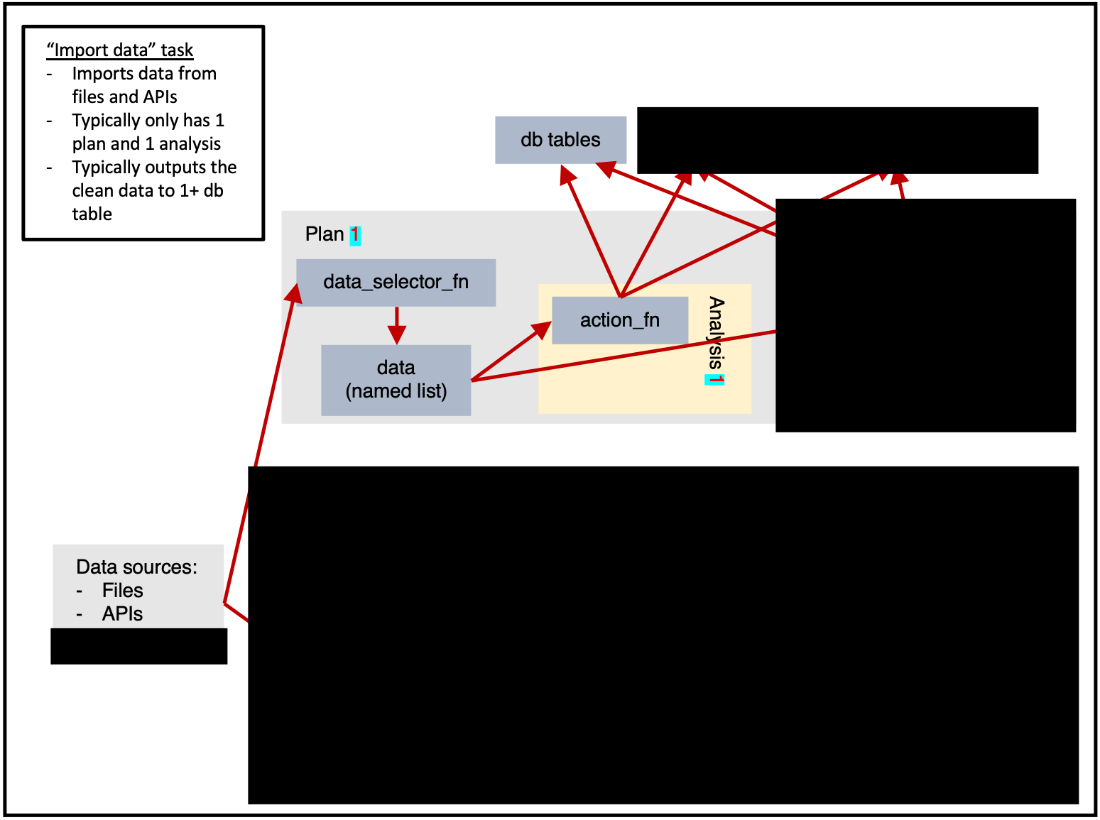
- Data Import Task: Download data from external APIs or files
- Data Cleaning Task: Validate, standardize, and quality-check incoming data
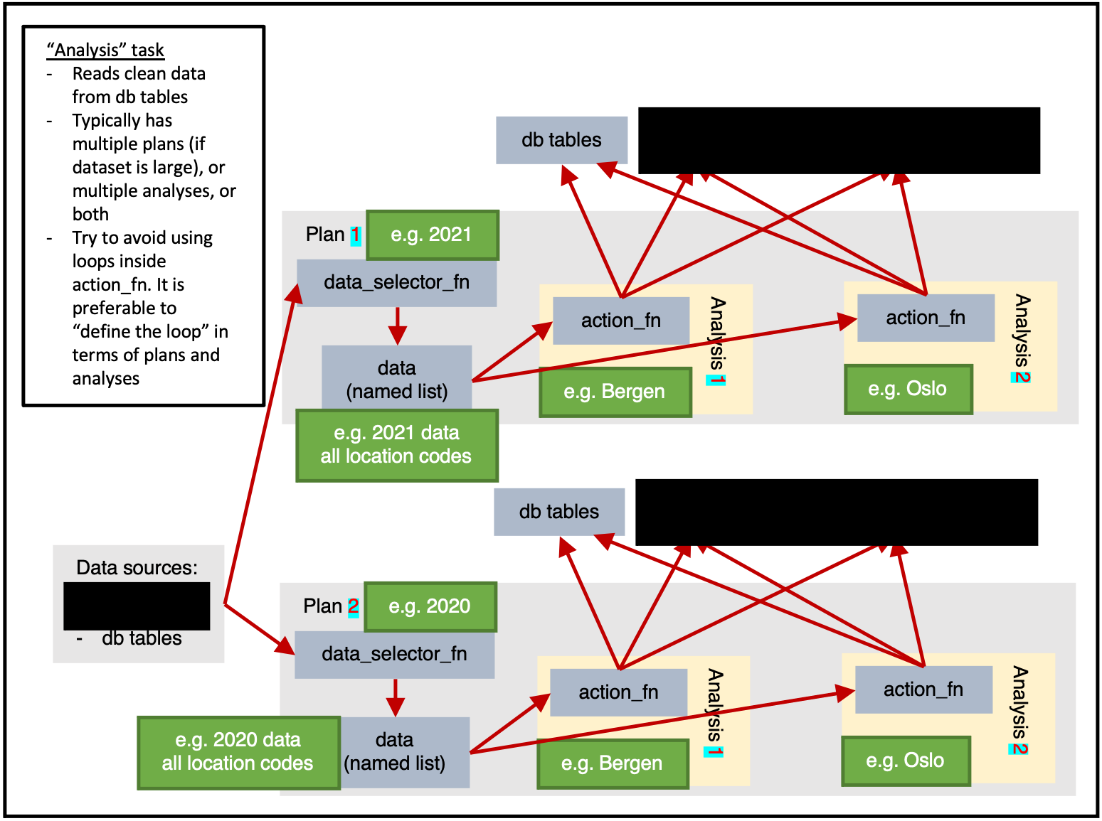
- Analysis Task: Calculate surveillance indicators, trends, or alerts
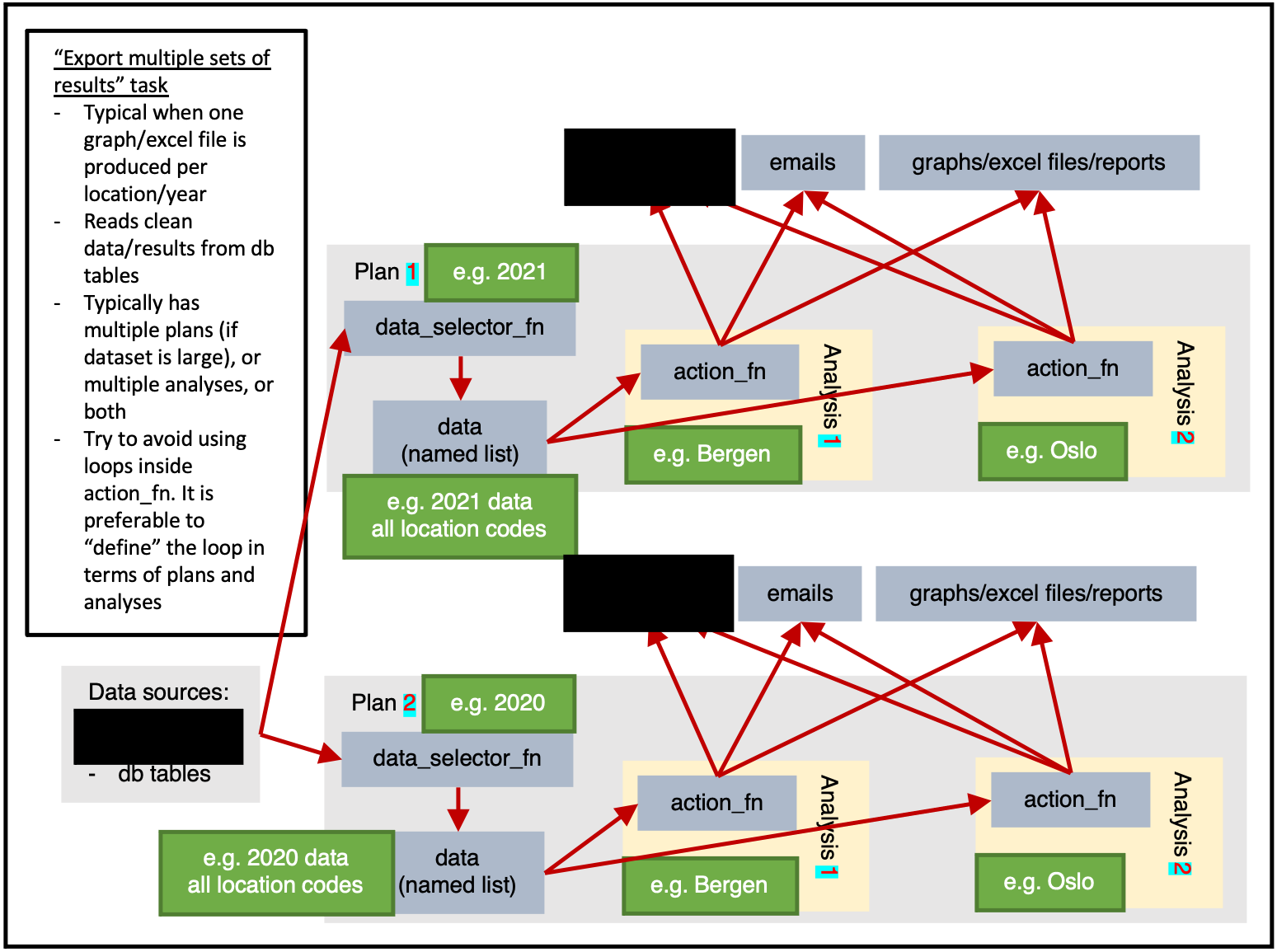
- Reporting Task: Generate outputs like Excel files, plots, or automated reports
- Delivery Task: Send results via email, upload to websites, or trigger alerts
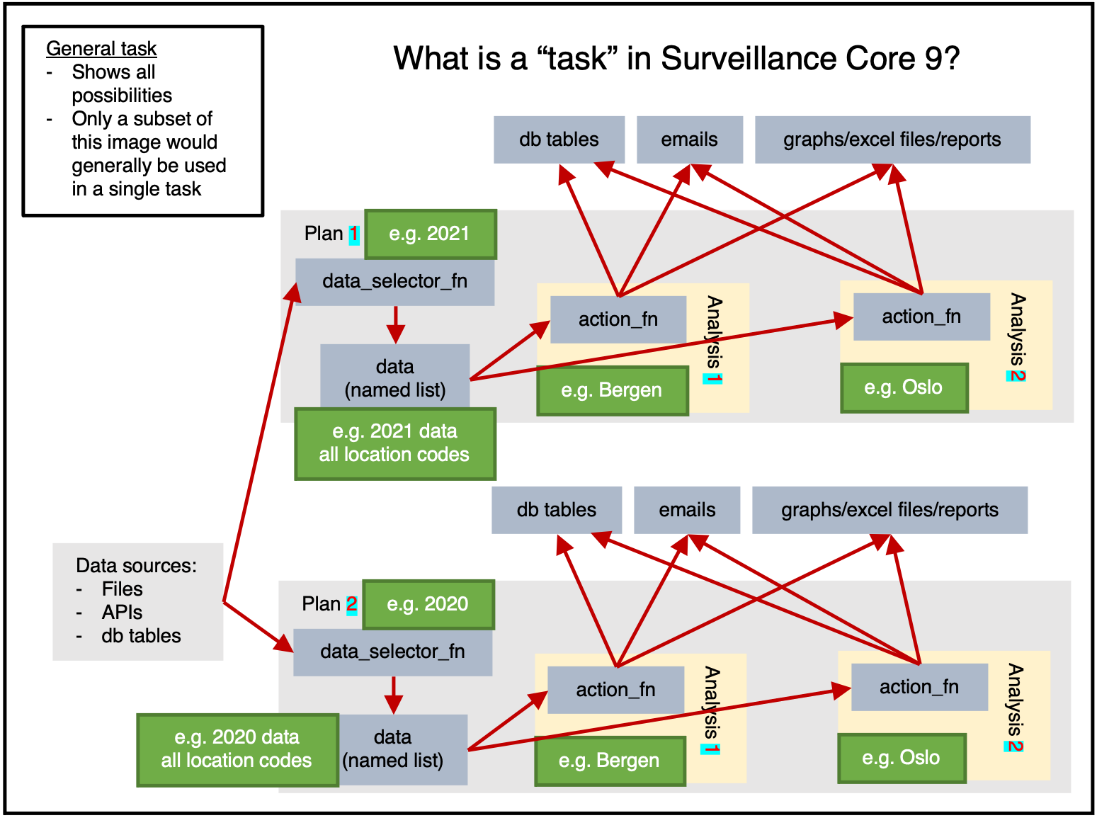
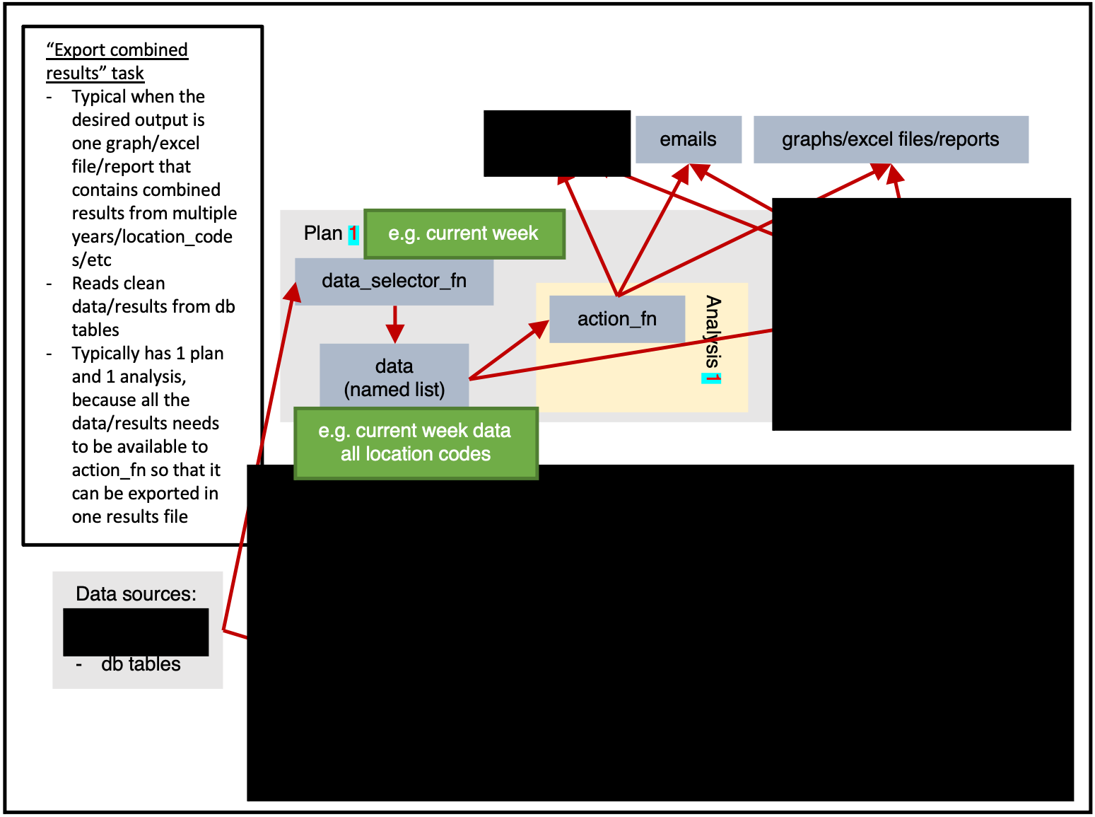
Figure 1 shows us the full potential of a task.
Data can be read from any sources, then within a plan the data will be extracted once by data_selector_fn (i.e. “one data-pull”). The data will then be provided to each analysis, which will run action_fn on:
- The provided data
- The provided argset
- The provided tables
The action_fn can then:
- Write data/results to db tables
- Send emails
- Export graphs, excel files, reports, or other physical files
Typically only a subset of this would be done in a single task.
Plan-heavy or analysis-heavy tasks?
A plan-heavy task is one that has many plans and a few analyses per plan.
An analysis-heavy task is one that has few plans and many analyses per plan.
In general, a data-pull is slow and wastes time. This means that it is preferable to reduce the number of data-pulls performed by having each data-pull extract larger quantities of data. The analysis can then subset the data as required (identifed via argsets). i.e. If possible, an analysis-heavy task is preferable because it will be faster (at the cost of needing more RAM).
Obviously, if a plan’s data-pull is larger, it will use more RAM. If you need to conserve RAM, then you should use a plan-heavy approach.
Figure 1 shows only 2 location based analyses, but in reality there are 356 municipalities in Norway in 2021. If figure 1 had 2 plans (1 for 2021 data, 1 for 2020 data) and 356 analyses for each plan (1 for each location_code) then we would be taking an analysis-heavy approach.
Getting Started with CS9
Now that you understand CS9’s architecture and concepts, you’re ready to start using it:
-
Installation and Setup: See
vignette("installation")for complete installation instructions, database configuration, and environment setup -
Package Structure: See
vignette("file-layout")for detailed guidance on organizing your CS9 implementation files
-
Creating Tasks: See
vignette("creating-a-task")for a step-by-step tutorial on implementing your first surveillance task
Example
We will now go through an example of how a person would design and implement a weather surveillance task.
Surveillance system setup
We begin by creating a surveillance system. This is the hub that coordinates everything.
ss <- cs9::SurveillanceSystem_v9$new()Database table definition
As documented in more detail here, we create a database table that fits our needs (recording weather data), and we then add it to the surveillance system.
ss$add_table(
  name_access = c("anon"),
  name_grouping = "example_weather",
  name_variant = NULL,
  field_types =  c(
    "granularity_time" = "TEXT",
    "granularity_geo" = "TEXT",
    "country_iso3" = "TEXT",
    "location_code" = "TEXT",
    "border" = "INTEGER",
    "age" = "TEXT",
    "sex" = "TEXT",

    "isoyear" = "INTEGER",
    "isoweek" = "INTEGER",
    "isoyearweek" = "TEXT",
    "season" = "TEXT",
    "seasonweek" = "DOUBLE",

    "calyear" = "INTEGER",
    "calmonth" = "INTEGER",
    "calyearmonth" = "TEXT",

    "date" = "DATE",

    "tg" = "DOUBLE",
    "tx" = "DOUBLE",
    "tn" = "DOUBLE"
  ),
  keys = c(
    "granularity_time",
    "location_code",
    "date",
    "age",
    "sex"
  ),
  validator_field_types = csdb::validator_field_types_csfmt_rts_data_v1,
  validator_field_contents = csdb::validator_field_contents_csfmt_rts_data_v1
)
Task configuration
To “register” our task, we use ss$add_task:
# tm_run_task("example_weather_import_data_from_api")
ss$add_task(
  name_grouping = "example_weather",
  name_action = "import_data_from_api",
  name_variant = NULL,
  cores = 1,
  plan_analysis_fn_name = NULL, # "PACKAGE::TASK_NAME_plan_analysis"
  for_each_plan = plnr::expand_list(
    location_code = "county03" # fhidata::norway_locations_names()[granularity_geo %in% c("county")]$location_code
  ),
  for_each_analysis = NULL,
  universal_argset = NULL,
  upsert_at_end_of_each_plan = FALSE,
  insert_at_end_of_each_plan = FALSE,
  action_fn_name = "example_weather_import_data_from_api_action",
  data_selector_fn_name = "example_weather_import_data_from_api_data_selector",
  tables = list(
    # input

    # output
    "anon_example_weather" = ss$tables$anon_example_weather
  )
)
There are a number of important things in this code that need highlighting.
for_each_plan
for_each_plan expects a list. Each component of the list will correspond to a plan, with the values added to the argset of all the analyses inside the plan.
For example, the following code would give 4 plans, with 1 analysis per each plan, with each analysis containing argset$var_1 and argset$var_2 as appropriate.
for_each_plan <- list()
for_each_plan[[1]] <- list(
  var_1 = 1,
  var_2 = "a"
)
for_each_plan[[2]] <- list(
  var_1 = 2,
  var_2 = "b"
)
for_each_plan[[3]] <- list(
  var_1 = 1,
  var_2 = "a"
)
for_each_plan[[4]] <- list(
  var_1 = 2,
  var_2 = "b"
)
You always need at least 1 plan. The most simple plan possible is:
plnr::expand_list(
  x = 1
)
#> [[1]]
#> [[1]]$x
#> [1] 1
plnr::expand_list
plnr::expand_list is esentially the same as expand.grid, except that its return values are lists instead of data.frame.
The code above could be simplified as follows.
for_each_plan <- plnr::expand_list(
  var_1 = c(1,2),
  var_2 = c("a", "b")
)
for_each_plan
#> [[1]]
#> [[1]]$var_1
#> [1] 1
#>
#> [[1]]$var_2
#> [1] "a"
#>
#>
#> [[2]]
#> [[2]]$var_1
#> [1] 2
#>
#> [[2]]$var_2
#> [1] "a"
#>
#>
#> [[3]]
#> [[3]]$var_1
#> [1] 1
#>
#> [[3]]$var_2
#> [1] "b"
#>
#>
#> [[4]]
#> [[4]]$var_1
#> [1] 2
#>
#> [[4]]$var_2
#> [1] "b"
for_each_analysis
for_each_plan expects a list, which will generate length(for_each_plan) plans.
for_each_analysis is the same, except it will generate analyses within each of the plans.
upsert_at_end_of_each_plan
If TRUE and tables contains a table called output, then the returned values of action_fn will be stored and upserted to tables$output at the end of each plan.
If TRUE and the returned values of action_fn are named lists, then the values within the named lists will be stored and upserted to tables$NAME_FROM_LIST at the end of each plan.
If you choose to upsert/insert manually from within action_fn, you can only do so at the end of each analysis.
insert_at_end_of_each_plan
If TRUE and tables contains a table called output, then the returned values of action_fn will be stored and inserted to tables$output at the end of each plan.
If TRUE and the returned values of action_fn are named lists, then the values within the named lists will be stored and inserted to tables$NAME_FROM_LIST at the end of each plan.
If you choose to upsert/insert manually from within action_fn, you can only do so at the end of each analysis.
data_selector_fn
The data_selector_fn is used to extract the data for each plan.
The lines inside if(plnr::is_run_directly()){ are used to help developers. You can run the code manually/interactively to “load” the values of argset and schema.
index_plan <- 1

argset <- ss$shortcut_get_argset("example_weather_import_data_from_api", index_plan = index_plan)
tables <- ss$shortcut_get_tables("example_weather_import_data_from_api")

print(argset)
#> $`**universal**`
#> [1] "*"
#>
#> $`**plan**`
#> [1] "*"
#>
#> $location_code
#> [1] "county03"
#>
#> $`**analysis**`
#> [1] "*"
#>
#> $`**automatic**`
#> [1] "*"
#>
#> $index
#> [1] 1
#>
#> $today
#> [1] "2025-08-21"
#>
#> $yesterday
#> [1] "2025-08-20"
#>
#> $index_plan
#> [1] 1
#>
#> $index_analysis
#> [1] 1
#>
#> $first_analysis
#> [1] TRUE
#>
#> $last_analysis
#> [1] TRUE
#>
#> $within_plan_first_analysis
#> [1] TRUE
#>
#> $within_plan_last_analysis
#> [1] TRUE
print(tables)
#> $anon_example_weather
#> public.anon_example_weather (disconnected)
#>
#>   1: granularity_time (TEXT) (KEY)
#>   2: granularity_geo (TEXT)
#>   3: country_iso3 (TEXT)
#>   4: location_code (TEXT) (KEY)
#>   5: border (INTEGER)
#>   6: age (TEXT) (KEY)
#>   7: sex (TEXT) (KEY)
#>   8: isoyear (INTEGER)
#>   9: isoweek (INTEGER)
#>  10: isoyearweek (TEXT)
#>  11: season (TEXT)
#>  12: seasonweek (DOUBLE)
#>  13: calyear (INTEGER)
#>  14: calmonth (INTEGER)
#>  15: calyearmonth (TEXT)
#>  16: date (DATE) (KEY)
#>  17: tg (DOUBLE)
#>  18: tx (DOUBLE)
#>  19: tn (DOUBLE)
#>  20: auto_last_updated_datetime (DATETIME)
# **** data_selector **** ----
#' example_weather_import_data_from_api (data selector)
#' @param argset Argset
#' @param tables DB tables
#' @export
example_weather_import_data_from_api_data_selector = function(argset, tables){
  if(plnr::is_run_directly()){
    # global$ss$shortcut_get_plans_argsets_as_dt("example_weather_import_data_from_api")

    index_plan <- 1

    argset <- ss$shortcut_get_argset("example_weather_import_data_from_api", index_plan = index_plan)
    tables <- ss$shortcut_get_tables("example_weather_import_data_from_api")
  }

  # find the mid lat/long for the specified location_code
  gps <- fhimaps::norway_nuts3_map_b2020_default_dt[location_code == argset$location_code,.(
    lat = mean(lat),
    long = mean(long)
  )]

  # download the forecast for the specified location_code
  d <- httr::GET(glue::glue("https://api.met.no/weatherapi/locationforecast/2.0/classic?lat={gps$lat}&lon={gps$long}"), httr::content_type_xml())
  d <- xml2::read_xml(d$content)

  # The variable returned must be a named list
  retval <- list(
    "data" = d
  )
  retval
}
action_fn
The lines inside if(plnr::is_run_directly()){ are used to help developers. You can run the code manually/interactively to “load” the values of argset and schema.
index_plan <- 1
index_analysis <- 1

data <- ss$shortcut_get_data("example_weather_import_data_from_api", index_plan = index_plan)
argset <- ss$shortcut_get_argset("example_weather_import_data_from_api", index_plan = index_plan, index_analysis = index_analysis)
tables <- ss$shortcut_get_tables("example_weather_import_data_from_api")

print(data)
#> $data
#> {xml_document}
#> <weatherdata noNamespaceSchemaLocation="https://schema.api.met.no/schemas/weatherapi-0.4.xsd" created="2025-08-21T13:28:23Z" xmlns:xsi="http://www.w3.org/2001/XMLSchema-instance">
#> [1] <meta>\n  <model name="met_public_forecast" termin="2025-08-21T13:00:00Z" ...
#> [2] <product class="pointData">\n  <time datatype="forecast" from="2025-08-21 ...
#>
#> $hash
#> $hash$current
#> [1] "fa7c1fd90a6d9bf24040ae24919e6972"
#>
#> $hash$current_elements
#> $hash$current_elements$data
#> [1] "edf868d91cd1f5fe47b57b2aeb1d010d"
print(argset)
#> $`**universal**`
#> [1] "*"
#>
#> $`**plan**`
#> [1] "*"
#>
#> $location_code
#> [1] "county03"
#>
#> $`**analysis**`
#> [1] "*"
#>
#> $`**automatic**`
#> [1] "*"
#>
#> $index
#> [1] 1
#>
#> $today
#> [1] "2025-08-21"
#>
#> $yesterday
#> [1] "2025-08-20"
#>
#> $index_plan
#> [1] 1
#>
#> $index_analysis
#> [1] 1
#>
#> $first_analysis
#> [1] TRUE
#>
#> $last_analysis
#> [1] TRUE
#>
#> $within_plan_first_analysis
#> [1] TRUE
#>
#> $within_plan_last_analysis
#> [1] TRUE
print(tables)
#> $anon_example_weather
#> public.anon_example_weather (disconnected)
#>
#>   1: granularity_time (TEXT) (KEY)
#>   2: granularity_geo (TEXT)
#>   3: country_iso3 (TEXT)
#>   4: location_code (TEXT) (KEY)
#>   5: border (INTEGER)
#>   6: age (TEXT) (KEY)
#>   7: sex (TEXT) (KEY)
#>   8: isoyear (INTEGER)
#>   9: isoweek (INTEGER)
#>  10: isoyearweek (TEXT)
#>  11: season (TEXT)
#>  12: seasonweek (DOUBLE)
#>  13: calyear (INTEGER)
#>  14: calmonth (INTEGER)
#>  15: calyearmonth (TEXT)
#>  16: date (DATE) (KEY)
#>  17: tg (DOUBLE)
#>  18: tx (DOUBLE)
#>  19: tn (DOUBLE)
#>  20: auto_last_updated_datetime (DATETIME)
# **** action **** ----
#' example_weather_import_data_from_api (action)
#' @param data Data
#' @param argset Argset
#' @param tables DB tables
#' @export
example_weather_import_data_from_api_action <- function(data, argset, tables) {
  # tm_run_task("example_weather_import_data_from_api")

  if(plnr::is_run_directly()){
    # global$ss$shortcut_get_plans_argsets_as_dt("example_weather_import_data_from_api")

    index_plan <- 1
    index_analysis <- 1

    data <- ss$shortcut_get_data("example_weather_import_data_from_api", index_plan = index_plan)
    argset <- ss$shortcut_get_argset("example_weather_import_data_from_api", index_plan = index_plan, index_analysis = index_analysis)
    tables <- ss$shortcut_get_tables("example_weather_import_data_from_api")
  }

  # code goes here
  # special case that runs before everything
  if(argset$first_analysis == TRUE){

  }

  a <- data$data

  baz <- xml2::xml_find_all(a, ".//maxTemperature")
  res <- vector("list", length = length(baz))
  for (i in seq_along(baz)) {
    parent <- xml2::xml_parent(baz[[i]])
    grandparent <- xml2::xml_parent(parent)
    time_from <- xml2::xml_attr(grandparent, "from")
    time_to <- xml2::xml_attr(grandparent, "to")
    x <- xml2::xml_find_all(parent, ".//minTemperature")
    temp_min <- xml2::xml_attr(x, "value")
    x <- xml2::xml_find_all(parent, ".//maxTemperature")
    temp_max <- xml2::xml_attr(x, "value")
    res[[i]] <- data.frame(
      time_from = as.character(time_from),
      time_to = as.character(time_to),
      tx = as.numeric(temp_max),
      tn = as.numeric(temp_min)
    )
  }
  res <- rbindlist(res)
  res <- res[stringr::str_sub(time_from, 12, 13) %in% c("00", "06", "12", "18")]
  res[, date := as.Date(stringr::str_sub(time_from, 1, 10))]
  res[, N := .N, by = date]
  res <- res[N == 4]
  res <- res[
    ,
    .(
      tg = NA,
      tx = max(tx),
      tn = min(tn)
    ),
    keyby = .(date)
  ]

  # we look at the downloaded data
  print("Data after downloading")
  print(res)

  # we now need to format it
  res[, granularity_time := "day"]
  res[, sex := "total"]
  res[, age := "total"]
  res[, location_code := argset$location_code]
  res[, border := 2020]

  # fill in missing structural variables
  cstidy::set_csfmt_rts_data_v1(res)

  # we look at the downloaded data
  print("Data after missing structural variables filled in")
  print(res)

  # put data in db table
  # tables$TABLE_NAME$insert_data(d)
  tables$anon_example_weather$upsert_data(res)
  # tables$TABLE_NAME$drop_all_rows_and_then_upsert_data(d)

  # special case that runs after everything
  # copy to anon_web?
  if(argset$last_analysis == TRUE){
    # cs9::copy_into_new_table_where(
    #   table_from = "anon_X",
    #   table_to = "anon_web_X"
    # )
  }
}
Run the task
ss$run_task("example_weather_import_data_from_api")
#> task: example_weather_import_data_from_api
#> Running task=example_weather_import_data_from_api with plans=1 and analyses=1
#> plans=sequential, argset=sequential with cores=1
#>
#> [1] "Data after downloading"
#> Key: <date>
#>          date     tg    tx    tn
#>        <Date> <lgcl> <num> <num>
#> 1: 2025-08-22     NA  16.0   8.8
#> 2: 2025-08-23     NA  17.6   8.0
#> 3: 2025-08-24     NA  18.4   9.8
#> 4: 2025-08-25     NA  18.1   8.8
#> 5: 2025-08-26     NA  18.8   8.9
#> 6: 2025-08-27     NA  19.7   9.2
#> 7: 2025-08-28     NA  20.4  10.2
#> 8: 2025-08-29     NA  19.0  10.1
#> 9: 2025-08-30     NA  16.9  12.1
#> [1] "Data after missing structural variables filled in"
#>    granularity_time granularity_geo country_iso3 location_code border    age
#>              <char>          <char>       <char>        <char>  <int> <char>
#> 1:              day          county          nor      county03   2020  total
#> 2:              day          county          nor      county03   2020  total
#> 3:              day          county          nor      county03   2020  total
#> 4:              day          county          nor      county03   2020  total
#> 5:              day          county          nor      county03   2020  total
#> 6:              day          county          nor      county03   2020  total
#> 7:              day          county          nor      county03   2020  total
#> 8:              day          county          nor      county03   2020  total
#> 9:              day          county          nor      county03   2020  total
#>       sex isoyear isoweek isoyearweek season seasonweek calyear calmonth
#>    <char>   <int>   <int>      <char> <char>      <num>   <int>    <int>
#> 1:  total      NA      NA        <NA>   <NA>         NA      NA       NA
#> 2:  total      NA      NA        <NA>   <NA>         NA      NA       NA
#> 3:  total      NA      NA        <NA>   <NA>         NA      NA       NA
#> 4:  total      NA      NA        <NA>   <NA>         NA      NA       NA
#> 5:  total      NA      NA        <NA>   <NA>         NA      NA       NA
#> 6:  total      NA      NA        <NA>   <NA>         NA      NA       NA
#> 7:  total      NA      NA        <NA>   <NA>         NA      NA       NA
#> 8:  total      NA      NA        <NA>   <NA>         NA      NA       NA
#> 9:  total      NA      NA        <NA>   <NA>         NA      NA       NA
#>    calyearmonth       date     tg    tx    tn
#>          <char>     <Date> <lgcl> <num> <num>
#> 1:         <NA> 2025-08-22     NA  16.0   8.8
#> 2:         <NA> 2025-08-23     NA  17.6   8.0
#> 3:         <NA> 2025-08-24     NA  18.4   9.8
#> 4:         <NA> 2025-08-25     NA  18.1   8.8
#> 5:         <NA> 2025-08-26     NA  18.8   8.9
#> 6:         <NA> 2025-08-27     NA  19.7   9.2
#> 7:         <NA> 2025-08-28     NA  20.4  10.2
#> 8:         <NA> 2025-08-29     NA  19.0  10.1
#> 9:         <NA> 2025-08-30     NA  16.9  12.1
#> Error in super$upsert_data(newdata, drop_indexes, verbose): upsert_load_data_infile not validated in anon_example_weather. granularity_time
Different types of tasks
Importing data
ss$add_task(
  name_grouping = "example",
  name_action = "import_data",
  name_variant = NULL,
  cores = 1,
  plan_analysis_fn_name = NULL,
  for_each_plan = plnr::expand_list(
    x = 1
  ),
  for_each_analysis = NULL,
  universal_argset = list(
    folder = cs9::path("input", "example")
  ),
  upsert_at_end_of_each_plan = FALSE,
  insert_at_end_of_each_plan = FALSE,
  action_fn_name = "example_import_data_action",
  data_selector_fn_name = "example_import_data_data_selector",
  tables = list(
    # input

    # output
    "output" = ss$tables$output
  )
)
Analysis
ss$add_task(
  name_grouping = "example",
  name_action = "analysis",
  name_variant = NULL,
  cores = 1,
  plan_analysis_fn_name = NULL,
  for_each_plan = plnr::expand_list(
    location_code = csdata::nor_locations_names()[granularity_geo %in% c("county")]$location_code
  ),
  for_each_analysis = NULL,
  universal_argset = NULL,
  upsert_at_end_of_each_plan = FALSE,
  insert_at_end_of_each_plan = FALSE,
  action_fn_name = "example_analysis_action",
  data_selector_fn_name = "example_analysis_data_selector",
  tables = list(
    # input
    "input" = ss$tables$input,

    # output
    "output" = ss$tables
  )
)
Exporting multiple sets of results
ss$add_task(
  name_grouping = "example",
  name_action = "export_results",
  name_variant = NULL,
  cores = 1,
  plan_analysis_fn_name = NULL,
  for_each_plan = plnr::expand_list(
    location_code = csdata::nor_locations_names()[granularity_geo %in% c("county")]$location_code
  ),
  for_each_analysis = NULL,
  universal_argset = list(
    folder = cs9::path("output", "example")
  ),
  upsert_at_end_of_each_plan = FALSE,
  insert_at_end_of_each_plan = FALSE,
  action_fn_name = "example_export_results_action",
  data_selector_fn_name = "example_export_results_data_selector",
  tables = list(
    # input
    "input" = ss$tables$input

    # output
  )
)
Exporting combined results
ss$tables(
  name_grouping = "example",
  name_action = "export_results",
  name_variant = NULL,
  cores = 1,
  plan_analysis_fn_name = NULL,
  for_each_plan = plnr::expand_list(
    x = 1
  ),
  for_each_analysis = NULL,
  universal_argset = list(
    folder = cs9::path("output", "example"),
    granularity_geos = c("nation", "county")
  ),
  upsert_at_end_of_each_plan = FALSE,
  insert_at_end_of_each_plan = FALSE,
  action_fn_name = "example_export_results_action",
  data_selector_fn_name = "example_export_results_data_selector",
  tables = list(
    # input
    "input" = ss$tables$input

    # output
  )
)
Deployment patterns
CS9 systems typically follow this deployment pattern:
-
Development: Use
devtools::load_all()for interactive development -
Testing: Run individual tasks with
global$ss$run_task("task_name") - Production: Deploy in Docker containers with Airflow scheduling
- Monitoring: Use built-in logging and configuration tracking
Getting started
To implement your own surveillance system:
- Clone the cs9example repository
- Perform global find/replace on “cs9example” with your package name
- Modify the table definitions in
03_tables.Rfor your data - Update the task definitions in
04_tasks.Rfor your analyses - Implement your surveillance tasks following the established patterns
This approach ensures you start with a working, tested framework rather than building from scratch.
Next steps
- Evaluate CS9: Install from CRAN and explore the documentation
- Review cs9example: Study the complete example implementation
- Set up infrastructure: Configure database and environment
- Clone cs9example: Use it as a template for your surveillance system
- Customize: Modify the example for your specific surveillance needs
For detailed infrastructure setup, see the Installation vignette.
For learning how to create tasks, see the Creating a Task vignette.
For understanding the file organization, see the File Layout vignette.