Customize your maps
Richard Aubrey White, Chi Zhang
2021-01-15
Source:vignettes/customization.Rmd
customization.Rmd
library(csmaps)
#> csmaps 2025.8.20
#> https://www.csids.no/csmaps/
library(ggplot2)
library(data.table)
library(magrittr)
Colored maps
Automatic coloring by location_code
pd <- copy(csmaps::nor_county_map_b2024_split_dt)

q <- ggplot()
q <- q + csmaps::annotate_oslo_nor_map_bxxxx_split_dt()
q <- q + geom_polygon(
  data = pd,
  mapping = aes(
    x = long,
    y = lat,
    group = group,
    fill = location_code
  ),
  color="black",
  linewidth = 0.4
)
q <- q + theme_void()
q <- q + coord_quickmap()
q <- q + labs(title = "")
q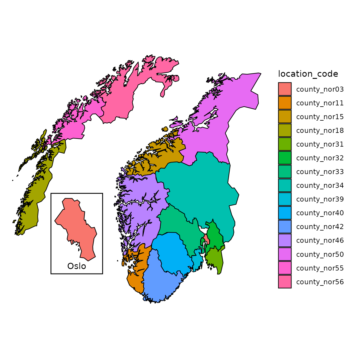
Customized coloring with external information
It is also possible to specify the color by user-defined groups. Here we show an example of assigning different (pseudo) risk level to each county.
pd <- copy(csmaps::nor_county_map_b2024_split_dt)

# assign each location a random category for different colors
location_info <- unique(pd[,c("location_code")])
location_info[,category:=rep(
  c("Good","Normal","Neutral","Bad","Very Bad"),
  each=3)[1:.N]
]
location_info[,category:=factor(
  category,
  levels=c("Good","Normal","Neutral","Bad","Very Bad")
  )
]
print(location_info)
#>     location_code category
#>            <char>   <fctr>
#>  1:  county_nor03     Good
#>  2:  county_nor11     Good
#>  3:  county_nor15     Good
#>  4:  county_nor18   Normal
#>  5:  county_nor31   Normal
#>  6:  county_nor32   Normal
#>  7:  county_nor33  Neutral
#>  8:  county_nor34  Neutral
#>  9:  county_nor39  Neutral
#> 10:  county_nor40      Bad
#> 11:  county_nor42      Bad
#> 12:  county_nor46      Bad
#> 13:  county_nor50 Very Bad
#> 14:  county_nor55 Very Bad
#> 15:  county_nor56 Very Bad

# join the map data.table
pd[
  location_info,
  on="location_code",
  category:=category
]

q <- ggplot()
q <- q + csmaps::annotate_oslo_nor_map_bxxxx_split_dt()
q <- q + geom_polygon(
  data = pd,
  mapping = aes(
    x = long,
    y = lat,
    group = group,
    fill = category
  ),
  color="black",
  linewidth = 0.4
)
q <- q + coord_quickmap()
q <- q + labs(title="")
q <- q + theme_void()
q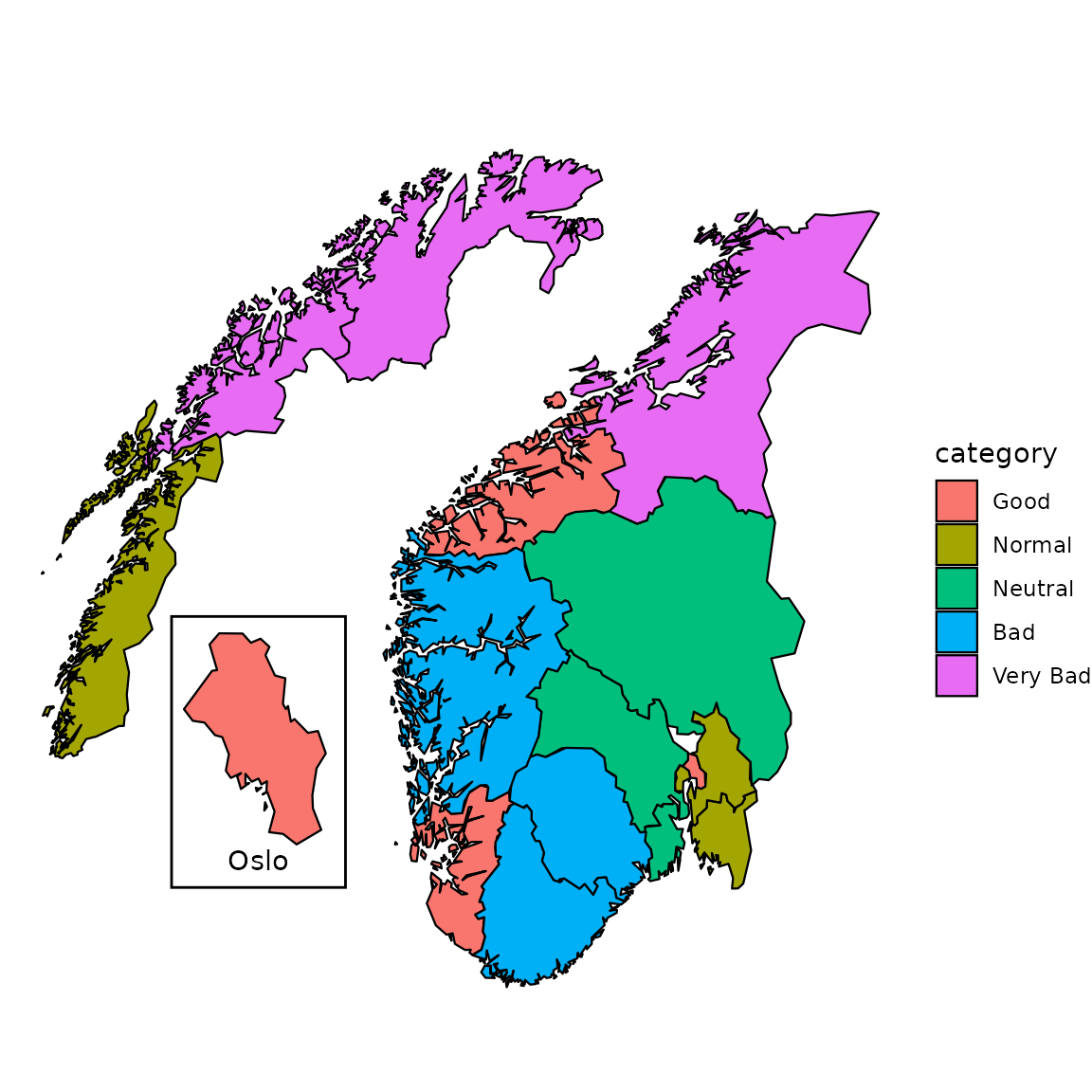
Labeled maps
We can add labels of county index onto the maps. There are several options for adding texts on a graph in ggplot2. We recommend geom_label() to add the labels if no label overlap occurs, otherwise we recommend using ggrepel::geom_label_repel().
q <- ggplot()
q <- q + csmaps::annotate_oslo_nor_map_bxxxx_split_dt()
q <- q + geom_polygon(
  data = pd,
  mapping = aes(
    x = long,
    y = lat,
    group = group,
    fill = category
  ),
  color="black",
  linewidth = 0.4
)
q <- q + geom_label(
  data = csmaps::nor_county_position_geolabels_b2024_split_dt,
  mapping = aes(
    x = long,
    y = lat,
    label = location_code
  )
)
# ggrepel::geom_label_repel() for avoiding overlap
q <- q + theme_void()
q <- q + coord_quickmap()
q <- q + labs(title = "")
q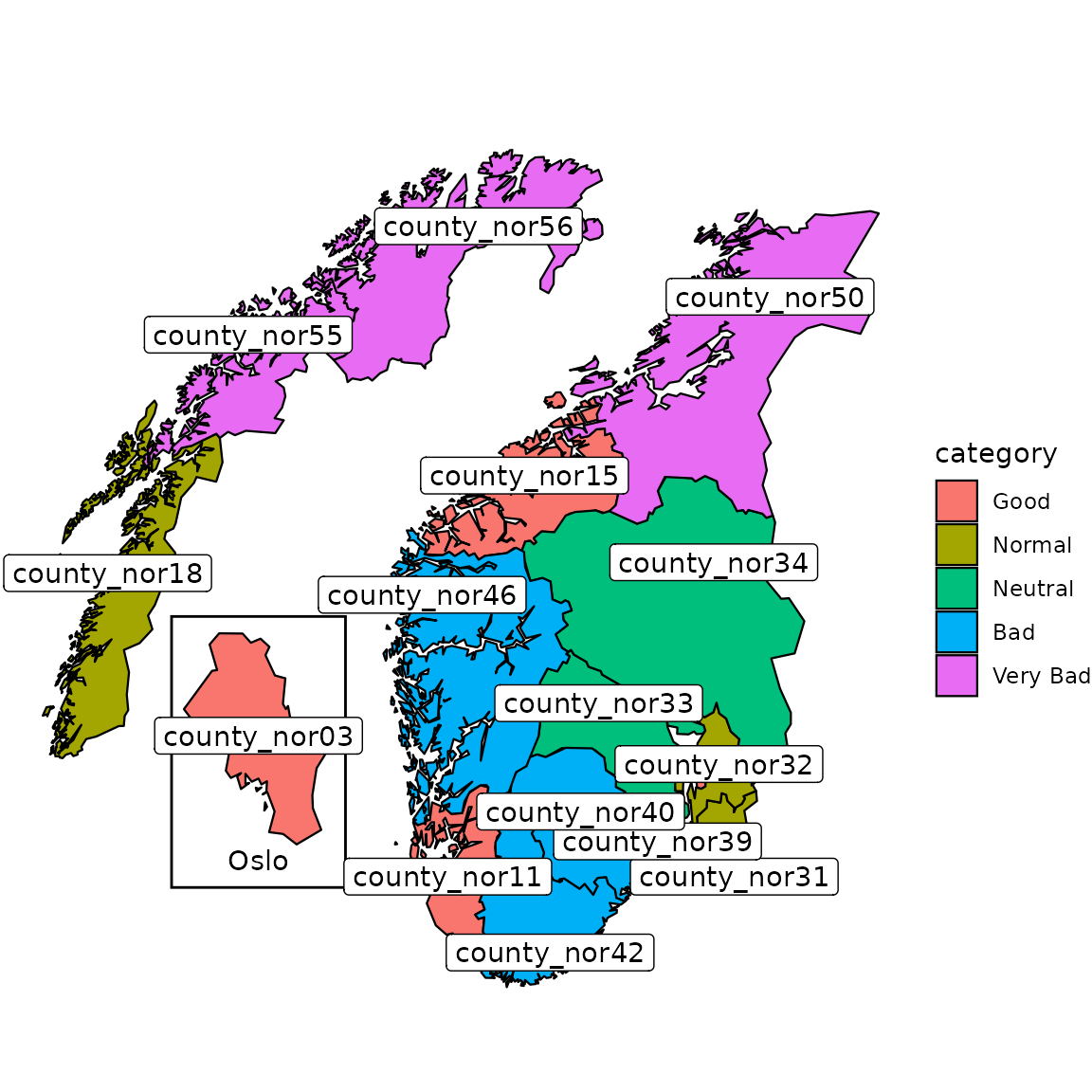
Labels can be easily added to other layouts, such as Oslo wards.
q <- ggplot(mapping = aes(x = long, y = lat))
q <- q + geom_polygon(
  data = csmaps::oslo_ward_map_b2024_default_dt,
  mapping = aes(group = group),
  color = "black",
  fill = "white",
  linewidth = 0.4
)
q <- q + geom_label(
  data = csmaps::oslo_ward_position_geolabels_b2024_default_dt,
  mapping = aes(label = location_code),
  color = "red",
  size = 3,
  label.size = 0.1,
  label.r = grid::unit(0, "lines")
)
q <- q + theme_void()
q <- q + coord_quickmap()
q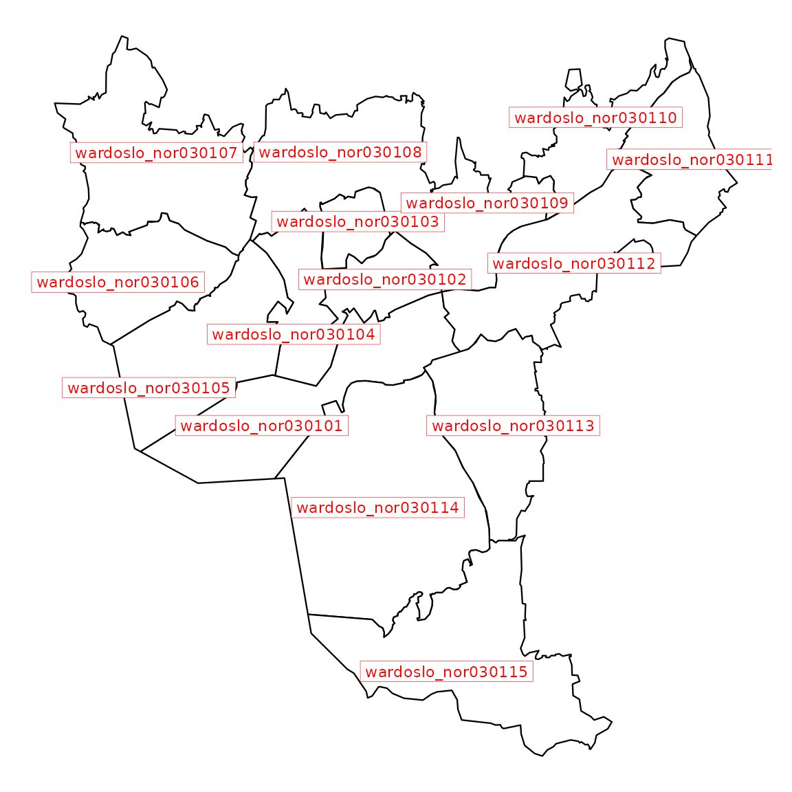
Enrich plot with additional data
It is convenient to use csdata package to enrich Norway and Oslo maps with external information, such as location name and population.
Add county name and population to Norway map
# enrich with population and location name
dpop_2024 <- csdata::nor_population_by_age_cats()[
  calyear==2024 &
  granularity_geo %in% "county"
]

# join, create label
labels <- copy(csmaps::nor_county_position_geolabels_b2024_split_dt)
labels[
  dpop_2024,
  on = "location_code",
  pop_total := pop_jan1_n
]
labels[
  csdata::nor_locations_names(),
  on = "location_code",
  location_name_short := location_name_short
]
labels[, label := paste0(location_name_short, '\n', pop_total)]
print(head(labels))
#>    location_code  long      lat  repel pop_total location_name_short
#>           <char> <num>    <num> <lgcl>     <num>              <char>
#> 1:  county_nor31 11.50 59.00000   TRUE    312152                 ØFO
#> 2:  county_nor32 11.20 60.03851   TRUE    728803                 AKR
#> 3:  county_nor33  8.85 60.60000   TRUE    269819                 BUS
#> 4:  county_nor03  2.20 60.30000  FALSE    717710                 OSL
#> 5:  county_nor34 11.10 61.90000  FALSE    376304                 INN
#> 6:  county_nor39 10.00 59.32481   TRUE    256432                 VFO
#>          label
#>         <char>
#> 1: ØFO\n312152
#> 2: AKR\n728803
#> 3: BUS\n269819
#> 4: OSL\n717710
#> 5: INN\n376304
#> 6: VFO\n256432

# plot
pd <- copy(csmaps::nor_county_map_b2024_split_dt)

q <- ggplot()
q <- q + csmaps::annotate_oslo_nor_map_bxxxx_split_dt()
q <- q + geom_polygon(
  data = pd,
  mapping = aes(
    x = long,
    y = lat,
    group = group,
    fill = location_code
  ),
  color="black",
  linewidth = 0.4
)
q <- q + ggrepel::geom_label_repel(
  data = labels[repel==TRUE],
  mapping = aes(x = long, y = lat, label = label),
  size = 3,
  label.size = 0.1,
  label.r = grid::unit(0, "lines"),
  min.segment.length = 0
)
q <- q + geom_label(
  data = labels[repel==FALSE],
  mapping = aes(x = long, y = lat, label = label),
  size = 3,
  label.size = 0.1,
  label.r = grid::unit(0, "lines")
)
q <- q + theme_void()
q <- q + coord_quickmap()
q <- q + labs(title = "")
q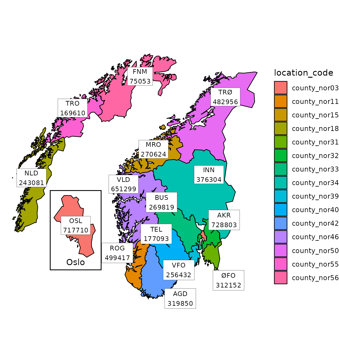
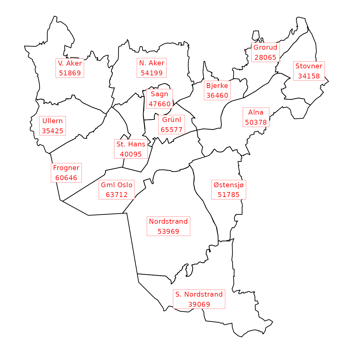
Add location name for ward and population for Oslo map
# enrich with population and location name
dpop_2024 <- csdata::nor_population_by_age_cats()[calyear==2024]

# join, create label
labels <- copy(csmaps::oslo_ward_position_geolabels_b2024_default_dt)
labels[
  dpop_2024,
  on = "location_code",
  pop_total := pop_jan1_n
]
labels[
  csdata::nor_locations_names(),
  on = "location_code",
  location_name_short := location_name_short
]
labels[, label := paste0(location_name_short, '\n', pop_total)]
print(head(labels))
#>         location_code     long      lat pop_total location_name_short
#>                <char>    <num>    <num>     <num>              <char>
#> 1: wardoslo_nor030101 10.72000 59.89000     63712            Gml Oslo
#> 2: wardoslo_nor030102 10.78000 59.92567     65577               Grünl
#> 3: wardoslo_nor030103 10.76683 59.93981     47660                Sagn
#> 4: wardoslo_nor030104 10.73555 59.91230     40095            St. Hans
#> 5: wardoslo_nor030105 10.66500 59.89925     60646             Frogner
#> 6: wardoslo_nor030106 10.65000 59.92500     35425              Ullern
#>              label
#>             <char>
#> 1: Gml Oslo\n63712
#> 2:    Grünl\n65577
#> 3:     Sagn\n47660
#> 4: St. Hans\n40095
#> 5:  Frogner\n60646
#> 6:   Ullern\n35425

q <- ggplot(mapping = aes(x = long, y = lat))
q <- q + geom_polygon(
  data = csmaps::oslo_ward_map_b2024_default_dt,
  mapping = aes(group = group),
  color = "black",
  fill = "white",
  linewidth = 0.4
)
q <- q + geom_label(
  data = labels,
  mapping = aes(label = label),
  color = "red",
  size = 3,
  label.size = 0.1,
  label.r = grid::unit(0, "lines")
)
q <- q + theme_void()
q <- q + coord_quickmap()
q