Overview
The csstyle package provides a system for standardizing outputs such as graphs, tables, and reports using CSIDS visual guidelines. Rather than offering infinite customization options, csstyle focuses on producing a limited set of outputs that consistently look the same.
Key Features
- Consistent ggplot2 themes with CSIDS styling
-
Predefined color palettes for professional visualizations
- Norwegian number formatting conventions
- Utility functions for common tasks
Using CSIDS Themes
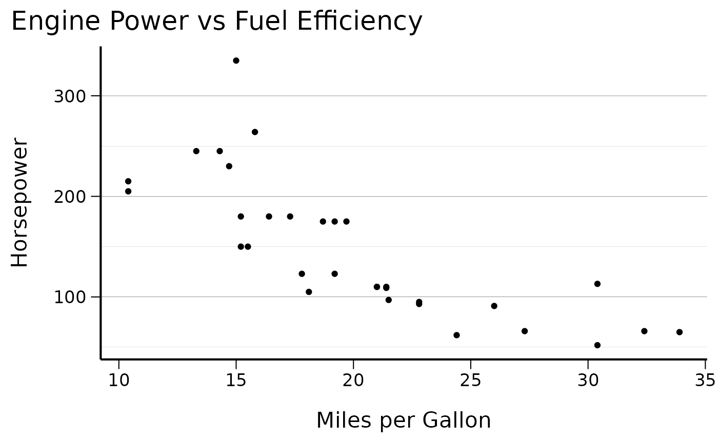
The main theme function theme_cs() provides a clean, professional appearance:
# Basic scatter plot with CSIDS theme
ggplot(mtcars, aes(x = mpg, y = hp)) +
  geom_point() +
  theme_cs() +
  labs(
    title = "Engine Power vs Fuel Efficiency",
    x = "Miles per Gallon",
    y = "Horsepower"
  )
You can customize the theme with various options:
# Theme with bottom legend and vertical x-axis labels
ggplot(mtcars, aes(x = factor(cyl), y = mpg, fill = factor(cyl))) +
  geom_boxplot() +
  theme_cs(legend_position = "bottom", x_axis_vertical = TRUE) +
  labs(title = "MPG by Number of Cylinders", fill = "Cylinders")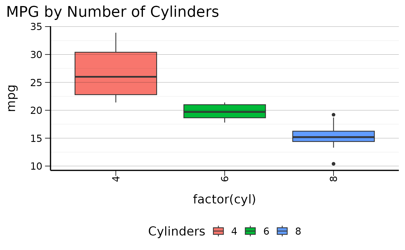
Color Palettes
The package includes several predefined color palettes:
# View available colors
head(colors$named_colors)
#>        H1        H2        H3        H4        H5        H6
#> "#393C61" "#0975B5" "#2EA1C0" "#709900" "#B11643" "#FC5F56"

# Display all palettes
display_all_palettes()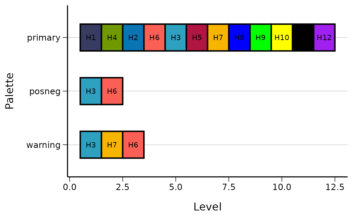
Use the color scales in your plots:
# Using the primary color palette
ggplot(mtcars, aes(x = mpg, y = hp, color = factor(cyl))) +
  geom_point(size = 3) +
  scale_color_cs(palette = "primary") +
  theme_cs() +
  labs(color = "Cylinders")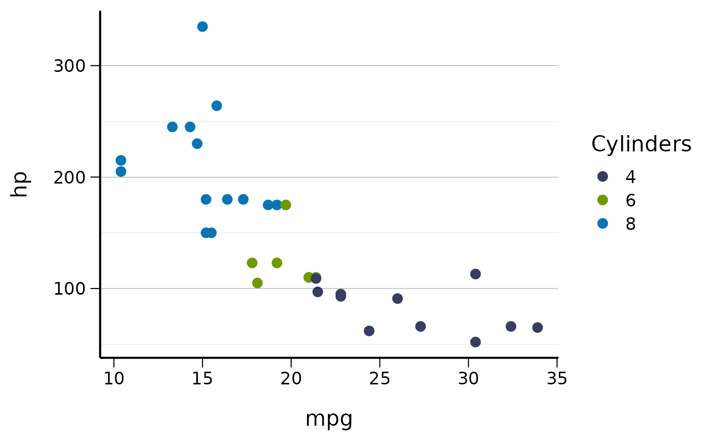
# Using the warning palette for fills
ggplot(mtcars, aes(x = factor(cyl), fill = factor(cyl))) +
  geom_bar() +
  scale_fill_cs(palette = "warning") +
  theme_cs() +
  labs(title = "Car Count by Cylinders", fill = "Cylinders")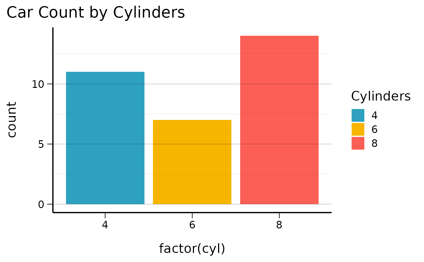
Number Formatting
The package provides Norwegian number formatting conventions:
# Format numbers with Norwegian conventions
numbers <- c(1234.56, 9876.54, 123.45, NA)

# Basic number formatting (0, 1, 2 decimal places)
format_num_as_nor_num_0(numbers)
#> [1] "1235" "9877" "123"  "IK"
format_num_as_nor_num_1(numbers)
#> [1] "1234,6" "9876,5" "123,5"  "IK"
format_num_as_nor_num_2(numbers)
#> [1] "1234,56" "9876,54" "123,45"  "IK"

# Percentage formatting
percentages <- c(12.34, 56.78, 90.12)
format_num_as_nor_perc_1(percentages)
#> [1] "12,3 %" "56,8 %" "90,1 %"

# Per 100k population rates
rates <- c(123.45, 678.90)
format_num_as_nor_per100k_1(rates)
#> [1] "123,5 /100k" "678,9 /100k"
Date Formatting
Format dates using Norwegian conventions:
# Current date
format_date_as_nor()
#> [1] "21.08.2025"

# Specific dates
test_date <- as.Date("2023-12-25")
format_date_as_nor(test_date)
#> [1] "25.12.2023"

# Datetime formatting
test_datetime <- as.POSIXct("2023-12-25 14:30:00")
format_datetime_as_nor(test_datetime)
#> [1] "25.12.2023 kl. 14:00"

# Filename-safe datetime
format_datetime_as_file(test_datetime)
#> [1] "2023_12_25_143000"
Journal Formatting
For academic publications, the package also provides journal formatting functions that use international conventions (comma thousands separator, decimal point, ISO 8601 dates):
Number Formatting Comparison
# Compare Norwegian vs Journal formatting
numbers <- c(1234.56, 9876.54, NA)

# Norwegian format (space thousands, comma decimal, "IK" for NA)
format_num_as_nor_num_1(numbers)
#> [1] "1234,6" "9876,5" "IK"

# Journal format (comma thousands, decimal point, "NA" for NA)
format_num_as_journal_num_1(numbers)
#> [1] "1,234.6" "9,876.5" "NA"

# Percentage comparison
percentages <- c(12.34, 56.78)

# Norwegian: "12,3 %" vs Journal: "12.3%"
format_num_as_nor_perc_1(percentages)
#> [1] "12,3 %" "56,8 %"
format_num_as_journal_perc_1(percentages)
#> [1] "12.3%" "56.8%"

# Per 100k comparison
rates <- c(123.45, 678.90)

# Norwegian: "123,5 /100k" vs Journal: "123.5/100k"
format_num_as_nor_per100k_1(rates)
#> [1] "123,5 /100k" "678,9 /100k"
format_num_as_journal_per100k_1(rates)
#> [1] "123.5/100k" "678.9/100k"
Date Formatting Comparison
test_date <- as.Date("2023-12-25")
test_datetime <- as.POSIXct("2023-12-25 14:30:00")

# Norwegian format: "25.12.2023"
format_date_as_nor(test_date)
#> [1] "25.12.2023"

# Journal format (ISO 8601): "2023-12-25"
format_date_as_journal(test_date)
#> [1] "2023-12-25"

# Datetime comparison
format_datetime_as_nor(test_datetime)     # "25.12.2023 kl. 14:00"
#> [1] "25.12.2023 kl. 14:00"
format_datetime_as_journal(test_datetime)  # "2023-12-25 14:30:00"
#> [1] "2023-12-25 14:30:00"
Log Scale Transformations
Both Norwegian and journal formats support inverse log transformations:
log_values <- c(1, 2, 3)

# Log2 transformations (2^1, 2^2, 2^3 = 2, 4, 8)
format_num_as_nor_invlog2_1(log_values)      # "2,0", "4,0", "8,0"
#> [1] "2,0" "4,0" "8,0"
format_num_as_journal_invlog2_1(log_values)  # "2.0", "4.0", "8.0"
#> [1] "2.0" "4.0" "8.0"

# Log10 transformations (10^1, 10^2, 10^3 = 10, 100, 1000)
format_num_as_journal_invlog10_1(log_values) # "10.0", "100.0", "1,000.0"
#> [1] "10.0"    "100.0"   "1,000.0"
Utility Functions
Pretty Breaks
Use pretty_breaks() for nicely formatted axis breaks:
ggplot(mtcars, aes(x = mpg, y = hp)) +
  geom_point() +
  scale_y_continuous(breaks = pretty_breaks(n = 4)) +
  theme_cs()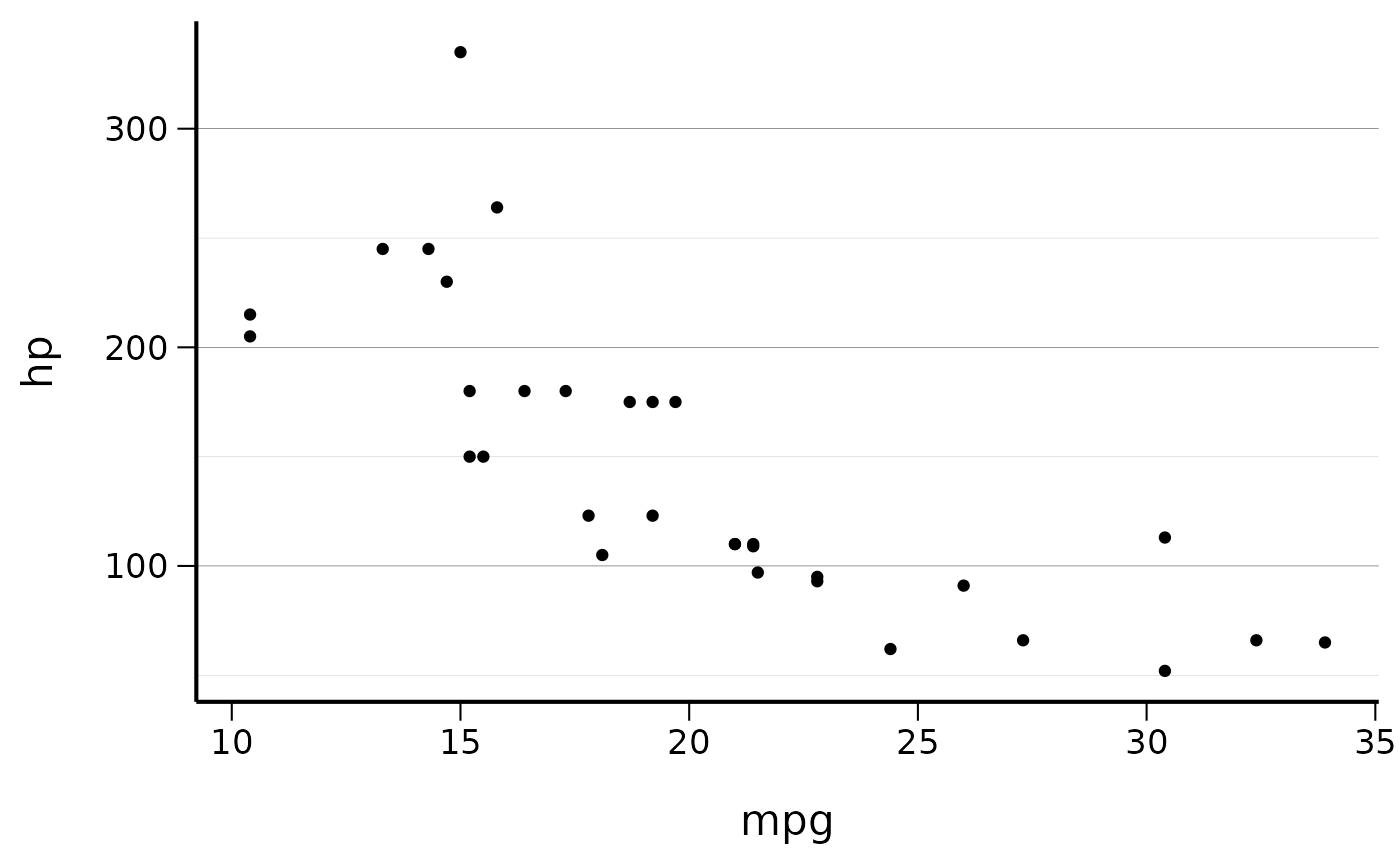
Every Nth
Display every nth label on crowded axes:
ggplot(mtcars, aes(x = rownames(mtcars), y = mpg)) +
  geom_col() +
  scale_x_discrete(breaks = every_nth(n = 4)) +
  theme_cs() +
  set_x_axis_vertical()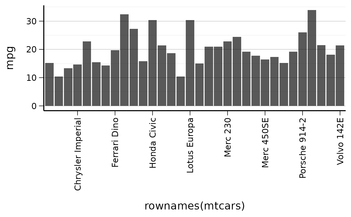
Conclusion
The csstyle package provides a comprehensive set of tools for creating consistent, professional visualizations that follow both Norwegian (CSIDS) and international journal standards. The dual formatting approach ensures that:
-
Norwegian functions (
*_as_nor) follow local conventions for domestic reports and presentations -
Journal functions (
*_as_journal) follow international standards for academic publications
By providing both options while limiting excessive customization, the package ensures consistent output formatting across different publication contexts.
For more detailed examples and function documentation, use help(package = "csstyle") or refer to individual function help pages.