# R CODE

library(data.table)
library(ggplot2)
set.seed(4)

AMPLITUDE <- 1.5
SEASONAL_HORIZONTAL_SHIFT <- 20

d <- data.table(date=seq.Date(
  from=as.Date("2000-01-01"),
  to=as.Date("2018-12-31"),
  by=1))
d[,year:=as.numeric(format.Date(date,"%G"))]
d[,week:=as.numeric(format.Date(date,"%V"))]
d[,month:=as.numeric(format.Date(date,"%m"))]
d[,yearMinus2000:=year-2000]
d[,dailyrainfall:=runif(.N, min=0, max=10)]

d[,dayOfYear:=as.numeric(format.Date(date,"%j"))]
d[,seasonalEffect:=sin(2*pi*(dayOfYear-SEASONAL_HORIZONTAL_SHIFT)/365)]
d[,mu := exp(0.1 + yearMinus2000*0.1 + seasonalEffect*AMPLITUDE)]
d[,y:=rpois(.N,mu)]2.1 Aim
We are given a dataset containing daily counts of diseases from one geographical area. We want to identify:
- Does seasonality exist?
- If seasonality exists, when are the high/low seasons?
- Is there a general yearly trend (i.e. increasing or decreasing from year to year?)
- Is daily rainfall associated with the number of cases?
2.2 Creating the data
The data for this chapter is available at: https://www.csids.no/longitudinal-analysis-for-surveillance/data/chapter_2.csv
2.3 True data
Here we show the true data, and note that there is an increasing annual trend (the data gets higher as time goes on) and there is a seasonal pattern (one peak/trough per year)
q <- ggplot(d,aes(x=date))
q <- q + geom_point(mapping=aes(y=y))
q <- q + geom_line(mapping=aes(y=mu),colour="red")
q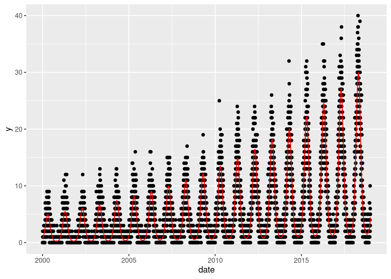
2.4 Investigation
Pretending we have no prior knowledge of our dataset, we display the data for few years and see a clear seasonal trend
q <- ggplot(d[year %in% c(2005:2010)],aes(x=dayOfYear,y=y))
q <- q + facet_wrap(~year)
q <- q + geom_point()
q <- q + stat_smooth(colour="red")
q
`geom_smooth()` using method = 'loess' and formula 'y ~ x'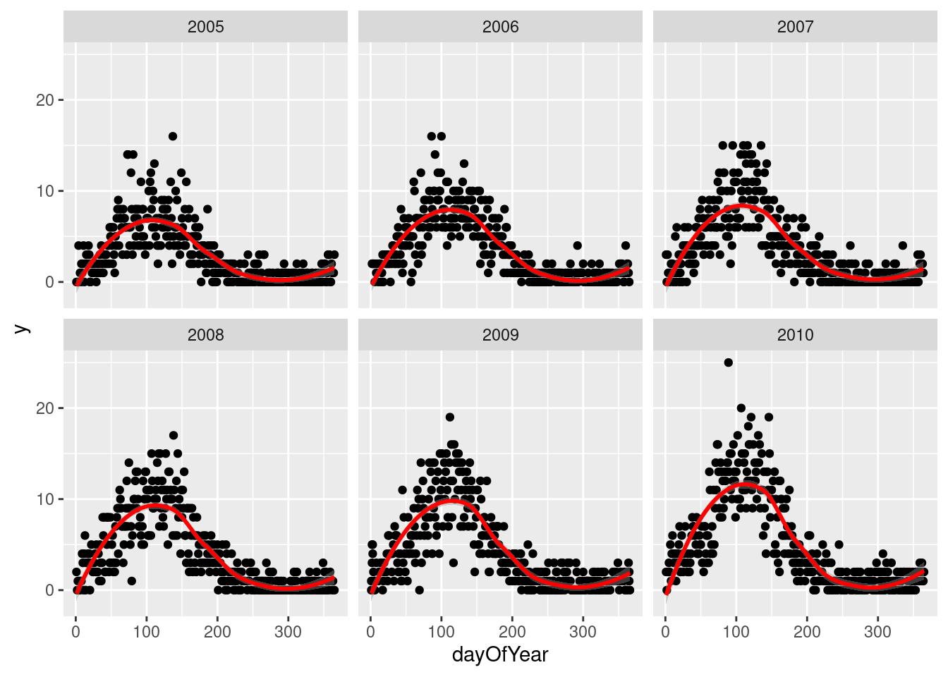
2.5 Seasonality
If we want to investigate the seasonality of our data, and identify when are the peaks and troughs, we have a few ways to approach this.
Non-parametric approaches are flexible and easy to implement, but they can lack power and be hard to interpret:
- Create a categorical variable for the seasons (e.g.
spring,summer,autumn,winter) and include this in the regression model - Create a categorical variable for the months (e.g.
Jan,Feb, …,Dec) and include this in the regression model
Parametric approaches are more powerful but require more effort:
- Identify the periodicity of the seasonality (how many days between peaks?)
- Using trigonometry, transform
day of yearinto variables that appropriately model the observed periodicity - Obtain coefficient estimates
- Back-transform these estimates into human-understandable values (day of peak, day of trough)
The non-parametric approaches are simple and we will therefore not cover them in this course. We will briefly examine the parametric approach.
NOTE: You don’t always have to investigate seasonality! It depends entirely on what the purpose of your analysis is!
The Lomb-Scargle Periodogram shows a clear seasonality with a period of 365 days.
// STATA CODE STARTS
insheet using "chapter_3.csv", clear

sort date
gen time=_n
tsset time, daily

wntestb y

cumsp y, gen(cumulative_spec_dist)
gen period=_N/_n

browse cumulative_spec_dist period
// STATA CODE ENDS
# R CODE
lomb::lsp(d$y,from=100,to=500,ofac=1,type="period")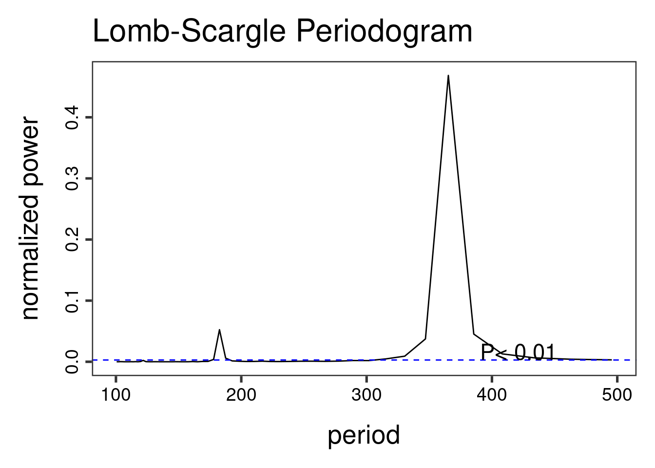
We then generate two new variables cos365 and sin365 and perform a likelihood ratio test to see if they are significant or not. This is done with two simple poisson regressions.
When we do not have autocorrelation, we can use the glm function in R and in STATA. Note that it is very important to specify the family (as this is how we differentiate between linear/logistic/poisson regressions).
// STATA CODE STARTS
gen cos365=cos(dayofyear*2*_pi/365)
gen sin365=sin(dayofyear*2*_pi/365)

glm y yearminus2000 dailyrainfall, family(poisson)
estimates store m1
glm y yearminus2000 dailyrainfall cos365 sin365, family(poisson)
estimates store m2

predict resid, anscombe

lrtest m1 m2
// STATA CODE ENDS
# R CODE
d[,cos365:=cos(dayOfYear*2*pi/365)]
d[,sin365:=sin(dayOfYear*2*pi/365)]
fit0 <- glm(y~yearMinus2000 + dailyrainfall, data=d, family=poisson())
fit1 <- glm(y~yearMinus2000 + dailyrainfall + sin365 + cos365, data=d, family=poisson())
print(lmtest::lrtest(fit0, fit1))Likelihood ratio test
Model 1: y ~ yearMinus2000 + dailyrainfall
Model 2: y ~ yearMinus2000 + dailyrainfall + sin365 + cos365
#Df LogLik Df Chisq Pr(>Chisq)
1 3 -26904
2 5 -12892 2 28024 < 2.2e-16 ***
---
Signif. codes: 0 '***' 0.001 '**' 0.01 '*' 0.05 '.' 0.1 ' ' 1We see that the likelihood ratio test for sin365 and cos365 was significant, meaning that there is significant seasonality with a 365 day periodicity in our data (which we already strongly suspected due to the periodogram).
We can now run/look at the results of our main regression.
print(summary(fit1))
Call:
glm(formula = y ~ yearMinus2000 + dailyrainfall + sin365 + cos365,
    family = poisson(), data = d)

Deviance Residuals:
    Min       1Q   Median       3Q      Max
-4.0676  -0.9229  -0.1170   0.5861   3.4103

Coefficients:
                Estimate Std. Error z value Pr(>|z|)
(Intercept)    0.0887436  0.0176742   5.021 5.14e-07 ***
yearMinus2000  0.1016117  0.0010525  96.539  < 2e-16 ***
dailyrainfall  0.0002287  0.0018476   0.124    0.901
sin365         1.3972586  0.0103200 135.393  < 2e-16 ***
cos365        -0.5035265  0.0086308 -58.341  < 2e-16 ***
---
Signif. codes:  0 '***' 0.001 '**' 0.01 '*' 0.05 '.' 0.1 ' ' 1

(Dispersion parameter for poisson family taken to be 1)

    Null deviance: 45536.8  on 6939  degrees of freedom
Residual deviance:  7328.5  on 6935  degrees of freedom
AIC: 25794

Number of Fisher Scoring iterations: 5
We also see that the (significant!) coefficient for year is 0.1 which means that for each additional year, the outcome increases by exp(0.1)=1.11. We also see that the coefficient for dailyrainfall was not significant, which means that we did not find a significant association between the outcome and dailyrainfall.
NOTE: See that this is basically the same as a normal regression.
Through the likelihood ratio test we saw a clear significant seasonal effect. We can now use trigonometry to back-calculate the amplitude and location of peak/troughs from the cos365 and sin365 estimates:
b1 <- 1.428417 # sin coefficient
b2 <- -0.512912 # cos coefficient
amplitude <- sqrt(b1^2 + b2^2)
p <- atan(b1/b2) * 365/2/pi
if (p > 0) {
    peak <- p
    trough <- p + 365/2
} else {
    peak <- p + 365/2
    trough <- p + 365
}
if (b1 < 0) {
    g <- peak
    peak <- trough
    trough <- g
}
print(sprintf("amplitude is estimated as %s, peak is estimated as %s, trough is estimated as %s",round(amplitude,2),round(peak),round(trough)))
[1] "amplitude is estimated as 1.52, peak is estimated as 111, trough is estimated as 294"print(sprintf("true values are: amplitude: %s, peak: %s, trough: %s",round(AMPLITUDE,2),round(365/4+SEASONAL_HORIZONTAL_SHIFT),round(3*365/4+SEASONAL_HORIZONTAL_SHIFT)))[1] "true values are: amplitude: 1.5, peak: 111, trough: 294"NOTE: An amplitude of 1.5 means that when comparing the average time of year to the peak, the peak is expected to be exp(1.5)=4.5 times higher than average. We take the exponential because we have run a poisson regression (so think incident rate ratio).
We now investigate our residuals to determine if we have a good fit:
d[,residuals:=residuals(fit1, type = "response")]
d[,predicted:=predict(fit1, type = "response")]
q <- ggplot(d,aes(x=predicted,y=residuals))
q <- q + geom_point()
q <- q + stat_smooth(colour="red")
q
`geom_smooth()` using method = 'gam' and formula 'y ~ s(x, bs = "cs")'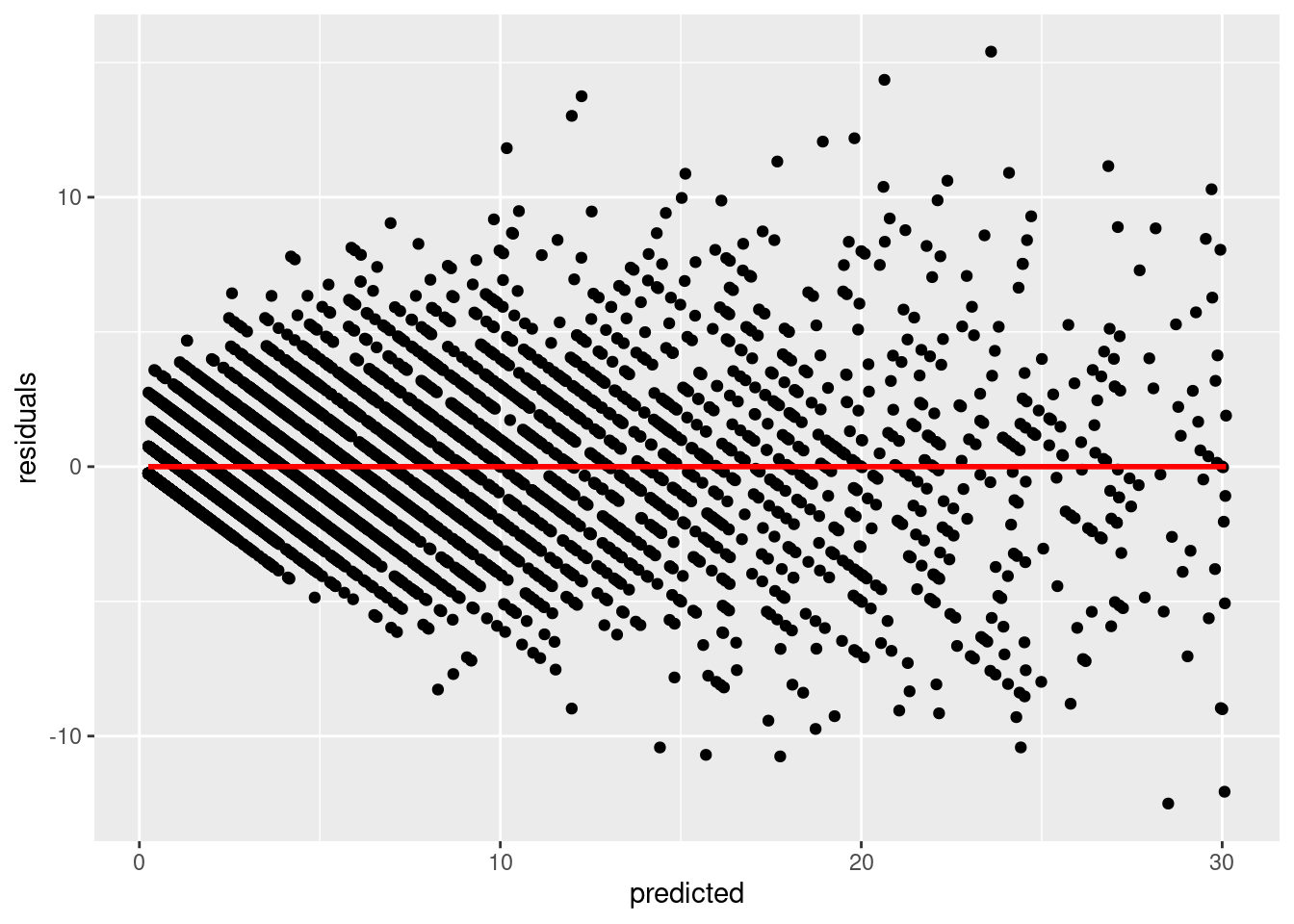
We check the pacf of the residuals to ensure that it is not AR. If we observe AR in our residuals, then this model was not appropriate and we need to use a different model.
// STATA CODE STARTS
pac resid
// STATA CODE ENDS
# R CODE
# this is for AR
pacf(d$residuals)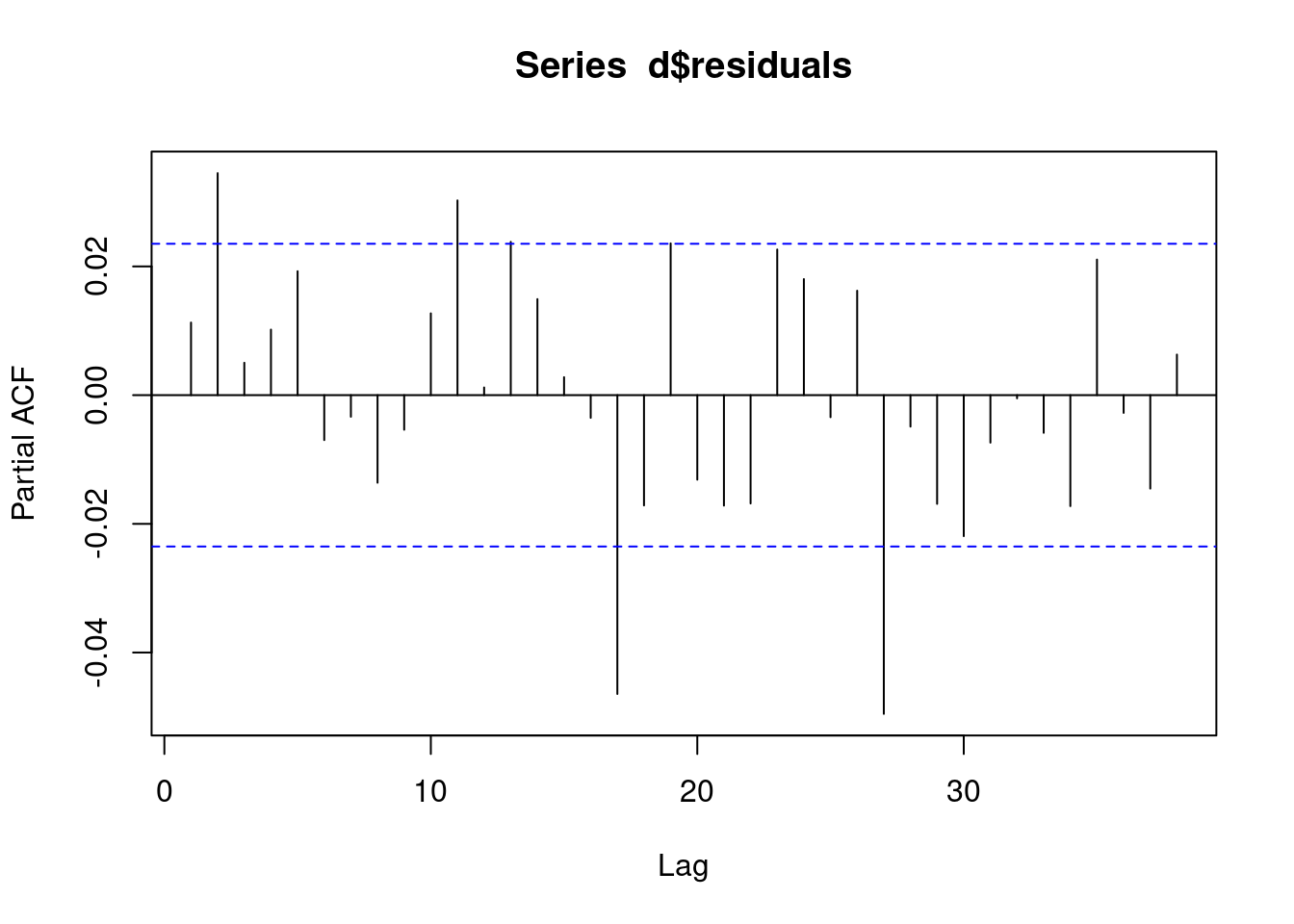
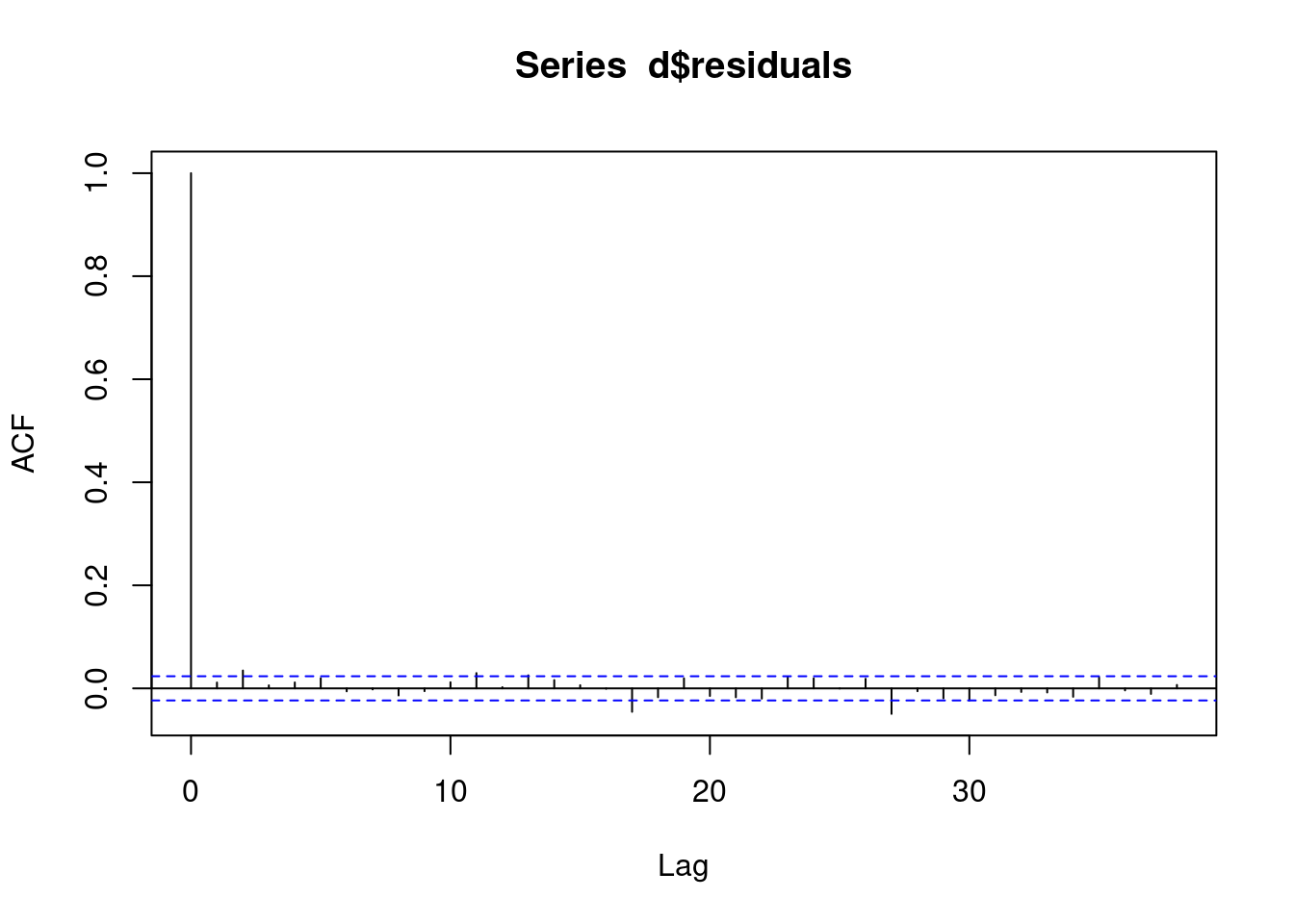
We check the acf of the residuals to ensure that it is not MA. If we observe MA in our residuals, then this model was not appropriate and we need to use a different model.
// STATA CODE STARTS
ac resid
// STATA CODE ENDS
# R CODE
# this is for MA
acf(d$residuals)