library(data.table)
library(ggplot2)
set.seed(4)

AMPLITUDE <- 1.5
SEASONAL_HORIZONTAL_SHIFT <- 20

d <- data.table(date=seq.Date(
  from=as.Date("2000-01-01"),
  to=as.Date("2018-12-31"),
  by=1))
d[,year:=as.numeric(format.Date(date,"%G"))]
d[,week:=as.numeric(format.Date(date,"%V"))]
d[,month:=as.numeric(format.Date(date,"%m"))]
d[,yearMinus2000:=year-2000]
d[,dayOfSeries:=1:.N]

d[,dayOfYear:=as.numeric(format.Date(date,"%j"))]
d[,seasonalEffect:=sin(2*pi*(dayOfYear-SEASONAL_HORIZONTAL_SHIFT)/365)]
d[,mu := exp(0.1 + yearMinus2000*0.1 + seasonalEffect*AMPLITUDE)]
d[,y:=rpois(.N,mu)]
d[,y:=round(as.numeric(arima.sim(model=list("ar"=c(0.5)), rand.gen = rpois, n=nrow(d), lambda=mu)))]3.1 Aim
We are given a dataset containing daily counts of diseases from one geographical area. We want to identify:
- Does seasonality exist?
- If seasonality exists, when are the high/low seasons?
- Is there a general yearly trend (i.e. increasing or decreasing from year to year?)
(We remove the question about rainfall in order to simplify and streamline the exercise)
3.2 Creating the data
The data for this chapter is available at: https://www.csids.no/longitudinal-analysis-for-surveillance/data/chapter_3.csv
3.3 Investigation
We display the data for few years and see a clear seasonal trend
q <- ggplot(d[year %in% c(2005:2010)],aes(x=dayOfYear,y=y))
q <- q + facet_wrap(~year)
q <- q + geom_point()
q <- q + stat_smooth(colour="red")
q
`geom_smooth()` using method = 'loess' and formula 'y ~ x'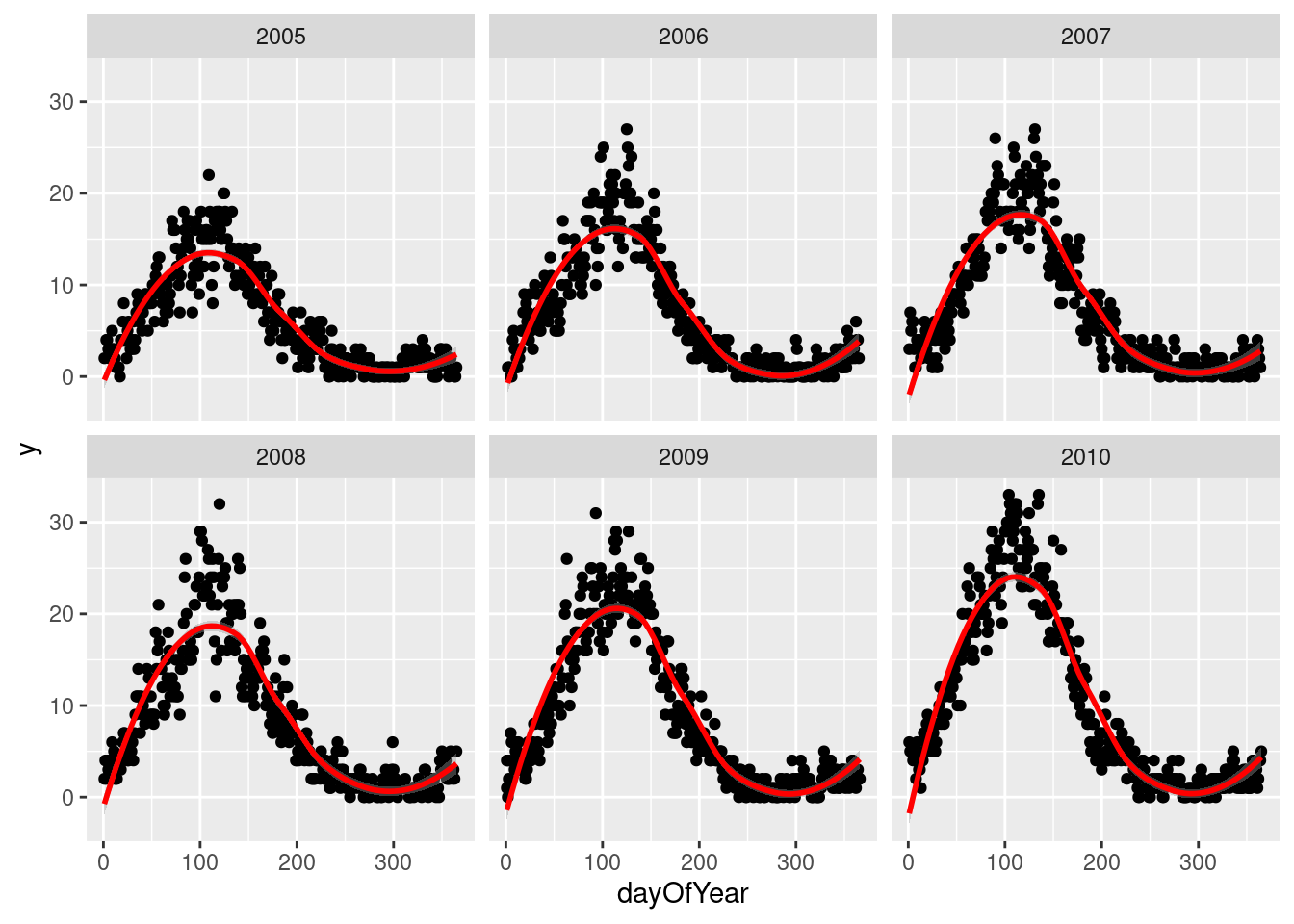
The Lomb-Scargle Periodogram shows a clear seasonality with a period of 365 days
// STATA CODE STARTS
insheet using "chapter_4.csv", clear

sort date
gen time=_n
tsset time, daily

wntestb y

cumsp y, gen(cumulative_spec_dist)
gen period=_N/_n

browse cumulative_spec_dist period
// STATA CODE ENDS
# R CODE
lomb::lsp(d$y,from=50,to=500,ofac=1,type="period")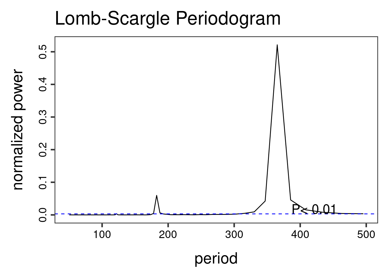
3.4 Regressions
We then generate two new variables cos365 and sin365 and perform a likelihood ratio test to see if they are significant or not. This is done with two simple poisson regressions.
// STATA CODE STARTS
gen cos365=cos(dayofyear*2*_pi/365)
gen sin365=sin(dayofyear*2*_pi/365)

glm y yearminus2000, family(poisson)
estimates store m1
glm y yearminus2000 cos365 sin365, family(poisson)
estimates store m2

predict resid, anscombe

lrtest m1 m2
// STATA CODE ENDS
# R CODE
d[,cos365:=cos(dayOfYear*2*pi/365)]
d[,sin365:=sin(dayOfYear*2*pi/365)]
fit0 <- glm(y~yearMinus2000, data=d, family=poisson())
fit1 <- glm(y~yearMinus2000+sin365 + cos365, data=d, family=poisson())
print(lmtest::lrtest(fit0, fit1))Likelihood ratio test
Model 1: y ~ yearMinus2000
Model 2: y ~ yearMinus2000 + sin365 + cos365
#Df LogLik Df Chisq Pr(>Chisq)
1 2 -43124
2 4 -14542 2 57163 < 2.2e-16 ***
---
Signif. codes: 0 '***' 0.001 '**' 0.01 '*' 0.05 '.' 0.1 ' ' 1We see that the likelihood ratio test for sin365 and cos365 was significant, meaning that there is significant seasonality with a 365 day periodicity in our data (which we already strongly suspected due to the periodogram).
We can now run/look at the results of our main regression.
print(summary(fit1))
Call:
glm(formula = y ~ yearMinus2000 + sin365 + cos365, family = poisson(),
    data = d)

Deviance Residuals:
    Min       1Q   Median       3Q      Max
-2.6774  -0.6738  -0.0503   0.4920   3.5820

Coefficients:
                Estimate Std. Error z value Pr(>|z|)
(Intercept)    0.7981246  0.0105300   75.80   <2e-16 ***
yearMinus2000  0.0991480  0.0007416  133.70   <2e-16 ***
sin365         1.4074818  0.0073418  191.71   <2e-16 ***
cos365        -0.5390314  0.0061513  -87.63   <2e-16 ***
---
Signif. codes:  0 '***' 0.001 '**' 0.01 '*' 0.05 '.' 0.1 ' ' 1

(Dispersion parameter for poisson family taken to be 1)

    Null deviance: 81832.6  on 6939  degrees of freedom
Residual deviance:  5217.8  on 6936  degrees of freedom
AIC: 29093

Number of Fisher Scoring iterations: 4
We also see that the coefficient for year is 0.1 which means that for each additional year, the outcome increases by exp(0.1)=1.11.
3.5 Residual analysis
d[,residuals:=residuals(fit1, type = "response")]
d[,predicted:=predict(fit1, type = "response")]
We can see a clear AR(1) pattern in our residuals.
// STATA CODE STARTS
pac resid
// STATA CODE ENDS
# R CODE
# this is for AR
pacf(d$residuals)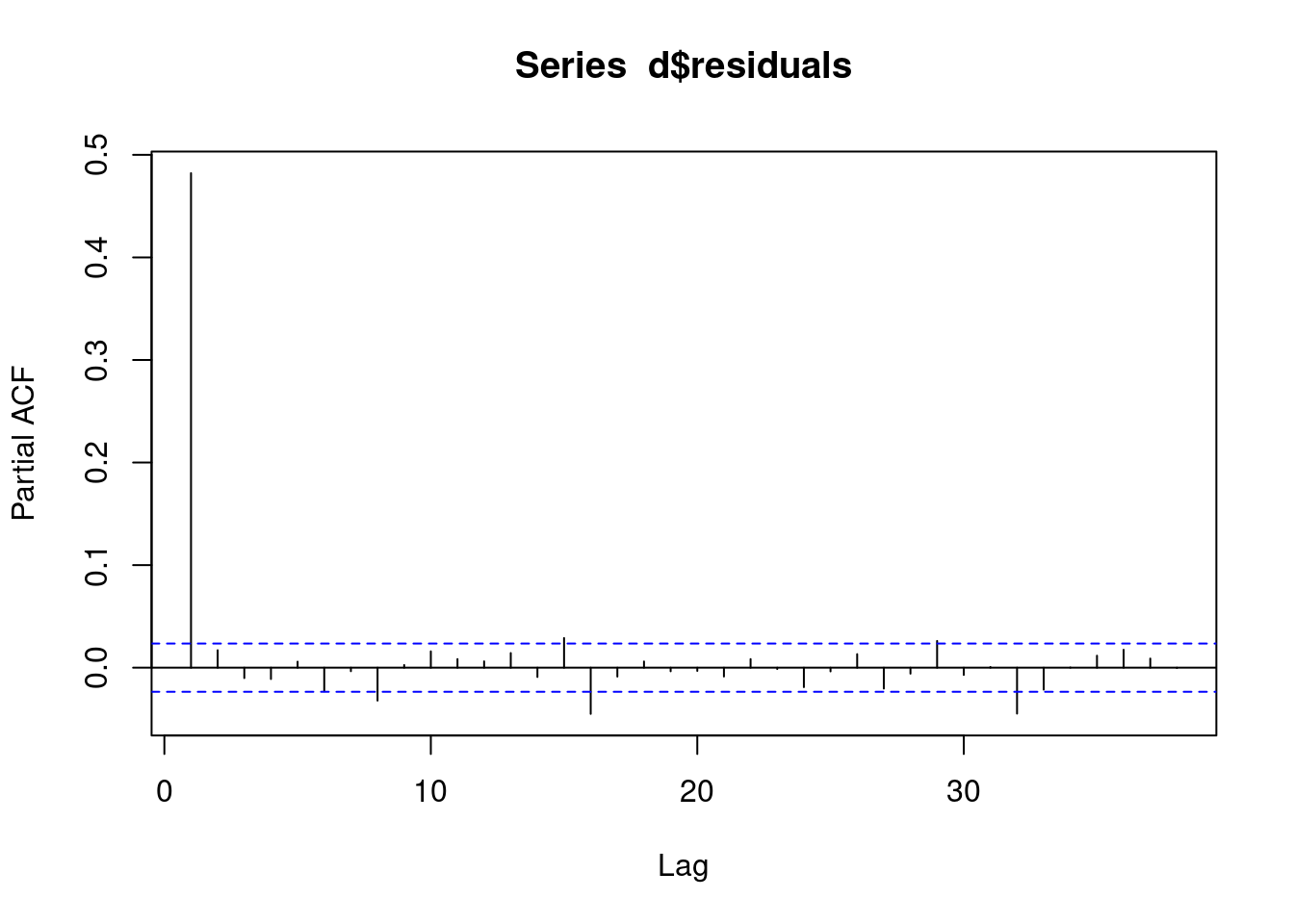
And again we see some sort of AR pattern in our residuals.
// STATA CODE STARTS
ac resid
// STATA CODE ENDS
# R CODE
# this is for MA
acf(d$residuals)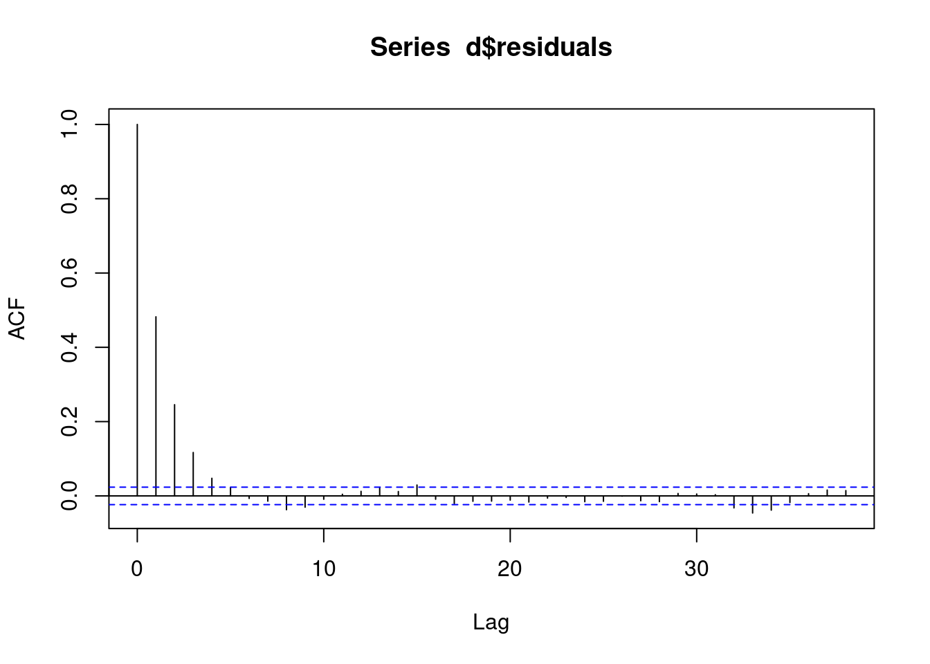
This means our model is bad, we have autocorrelation. We now need to change our model to account for this AR(1) autocorrelation!
3.6 (R ONLY) Regression with AR(1) correlation in residuals
First we create an id variable. This generally corresponds to geographical locations, or people. In this case, we only have one geographical location, so our id for all observations is 1. This lets the computer know that all data belongs to the same group.
When we have autocorrelation in the residuals, we can use the MASS::glmPQL function in R.
d[,ID:=1]
# this is for MA
fit <- MASS::glmmPQL(y~yearMinus2000+sin365 + cos365, random = ~ 1 | ID,
                family = poisson, data = d,
                correlation=nlme::corAR1(form=~dayOfSeries|ID))
iteration 1summary(fit)Linear mixed-effects model fit by maximum likelihood
Data: d
AIC BIC logLik
NA NA NA
Random effects:
Formula: ~1 | ID
(Intercept) Residual
StdDev: 1.149087e-05 0.841689
Correlation Structure: AR(1)
Formula: ~dayOfSeries | ID
Parameter estimate(s):
Phi
0.4926123
Variance function:
Structure: fixed weights
Formula: ~invwt
Fixed effects: y ~ yearMinus2000 + sin365 + cos365
Value Std.Error DF t-value p-value
(Intercept) 0.7980540 0.015203158 6936 52.49265 0
yearMinus2000 0.0991582 0.001070583 6936 92.62077 0
sin365 1.4074339 0.010596650 6936 132.81876 0
cos365 -0.5389807 0.008876448 6936 -60.72031 0
Correlation:
(Intr) yM2000 sin365
yearMinus2000 -0.832
sin365 -0.409 0.000
cos365 0.186 0.000 -0.158
Standardized Within-Group Residuals:
Min Q1 Med Q3 Max
-2.89886750 -0.75775061 -0.05982255 0.60730689 6.49964489
Number of Observations: 6940
Number of Groups: 1 We can see that the residuals no longer display any signs of autocorrelation.
pacf(residuals(fit, type = "normalized")) # this is for AR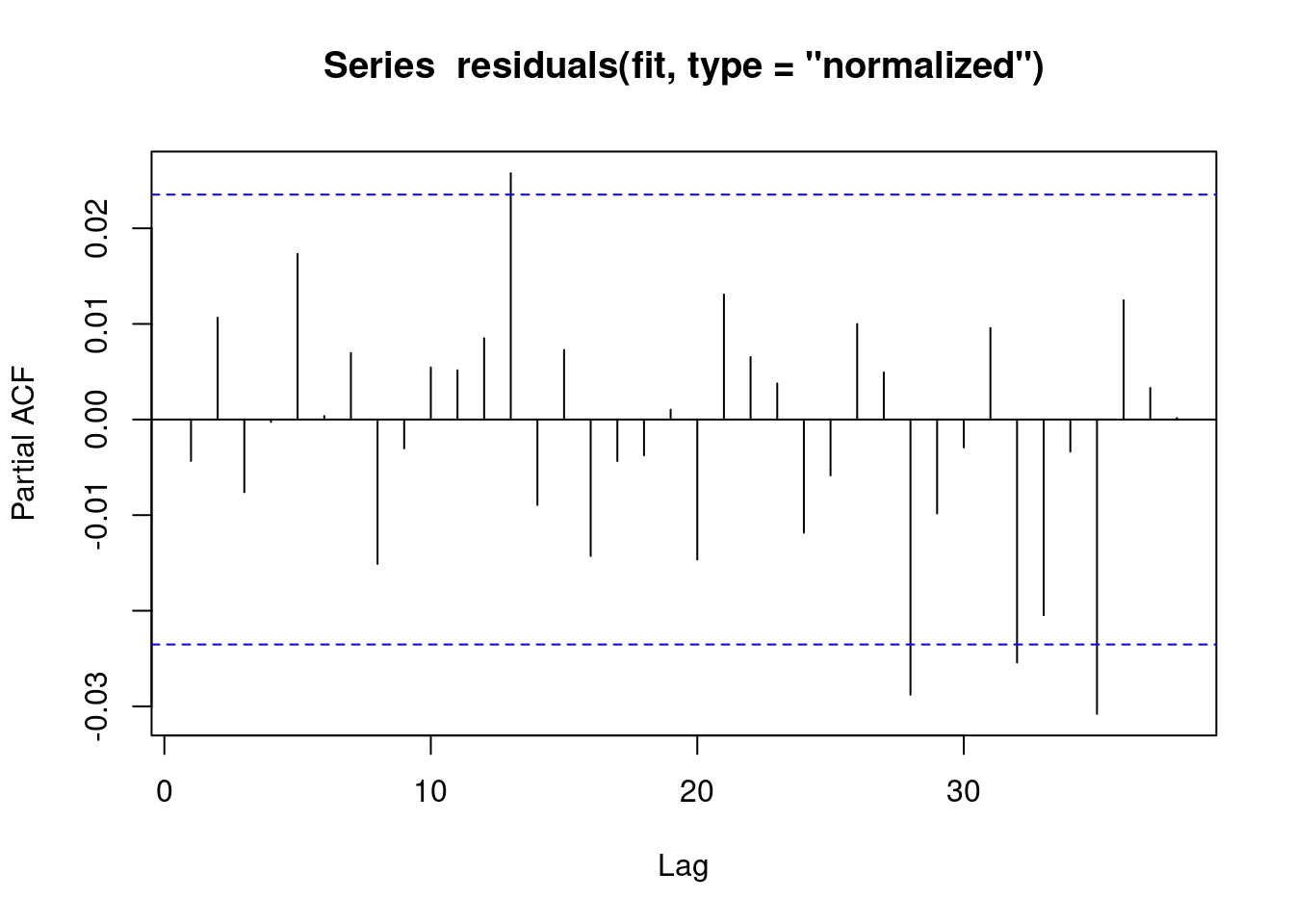
We can see that the residuals no longer display any signs of autocorrelation.
acf(residuals(fit, type = "normalized")) # this is for MA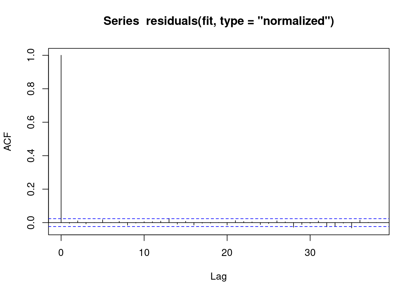
We also obtain the same estimates that we did in the last chapter.
b1 <- 1.3936185 # sin coefficient
b2 <- -0.5233866 # cos coefficient
amplitude <- sqrt(b1^2 + b2^2)
p <- atan(b1/b2) * 365/2/pi
if (p > 0) {
    peak <- p
    trough <- p + 365/2
} else {
    peak <- p + 365/2
    trough <- p + 365
}
if (b1 < 0) {
    g <- peak
    peak <- trough
    trough <- g
}
print(sprintf("amplitude is estimated as %s, peak is estimated as %s, trough is estimated as %s",round(amplitude,2),round(peak),round(trough)))
[1] "amplitude is estimated as 1.49, peak is estimated as 112, trough is estimated as 295"print(sprintf("true values are: amplitude: %s, peak: %s, trough: %s",round(AMPLITUDE,2),round(365/4+SEASONAL_HORIZONTAL_SHIFT),round(3*365/4+SEASONAL_HORIZONTAL_SHIFT)))[1] "true values are: amplitude: 1.5, peak: 111, trough: 294"3.7 (STATA ONLY) Regression with robust standard errors
In STATA it is not possible to explicitly model autocorrelation in the residuals (with the exception of linear regression). Since most of our work deals with logistic and poisson regressions, we will be focusing on modelling strategies that work with all kinds of regressions.
The STATA approach to autocorrelation is to estimate more robust standard errors. That is, STATA makes the standard errors larger to account for the model mispecification. This is done through the vce(robust) option.
// STATA CODE STARTS
glm y yearminus2000 cos365 sin365, family(poisson) vce(robust)
// STATA CODE ENDS