Likelihood ratio test

Model 1: y ~ yearMinus2000 + numberOfCows
Model 2: y ~ season + yearMinus2000 + numberOfCows
  #Df  LogLik Df  Chisq Pr(>Chisq)
1   3 -104814
2   6   -7847  3 193933  < 2.2e-16 ***
---
Signif. codes:  0 '***' 0.001 '**' 0.01 '*' 0.05 '.' 0.1 ' ' 1
summary(fit1)
Call:
glm(formula = y ~ season + yearMinus2000 + numberOfCows, family = poisson(),
    data = d)

Deviance Residuals:
    Min       1Q   Median       3Q      Max
-3.5547  -0.6743  -0.0203   0.6393   3.2527

Coefficients:
                Estimate Std. Error z value Pr(>|z|)
(Intercept)    0.0998769  0.0168980   5.911 3.41e-09 ***
seasonSpring   0.9996116  0.0077048 129.739  < 2e-16 ***
seasonSummer   2.0061609  0.0070148 285.990  < 2e-16 ***
seasonWinter  -0.0048955  0.0093124  -0.526    0.599
yearMinus2000  0.2001843  0.0011420 175.298  < 2e-16 ***
numberOfCows   0.1987005  0.0007667 259.153  < 2e-16 ***
---
Signif. codes:  0 '***' 0.001 '**' 0.01 '*' 0.05 '.' 0.1 ' ' 1

(Dispersion parameter for poisson family taken to be 1)

    Null deviance: 296600.3  on 2190  degrees of freedom
Residual deviance:   2167.4  on 2185  degrees of freedom
AIC: 15707

Number of Fisher Scoring iterations: 4
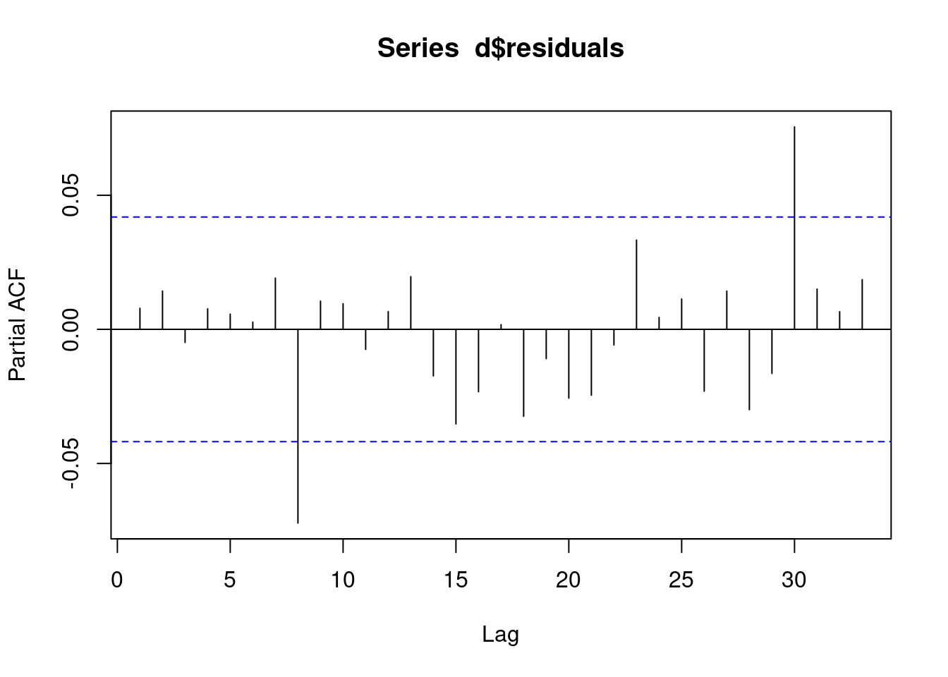
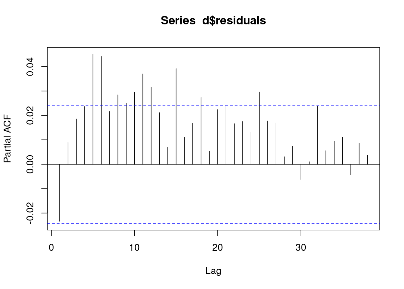
d[,residuals:=residuals(fit1, type ="response")]pacf(d$residuals)
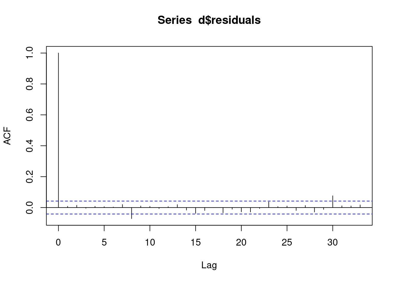
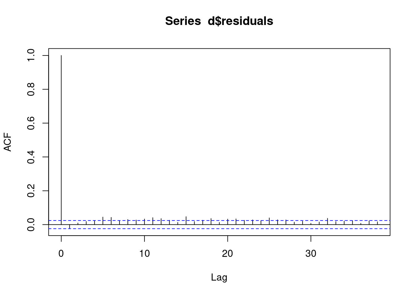
acf(d$residuals)
8.2 Exercise 2
library(data.table)d <-fread("data/exercise_2.csv")fit0 <- MASS::glmmPQL(y~yearMinus2000 + numberOfCows, random =~1| fylke,family = poisson, data = d)
iteration 1
iteration 2
fit1 <- MASS::glmmPQL(y~season + yearMinus2000 + numberOfCows, random =~1| fylke,family = poisson, data = d)
iteration 1
iteration 2
iteration 3
print(lmtest::lrtest(fit0, fit1))
Likelihood ratio test

Model 1: y ~ yearMinus2000 + numberOfCows
Model 2: y ~ season + yearMinus2000 + numberOfCows
  #Df LogLik Df Chisq Pr(>Chisq)
1   5
2   8         3
summary(fit1)
Linear mixed-effects model fit by maximum likelihood
  Data: d
  AIC BIC logLik
   NA  NA     NA

Random effects:
 Formula: ~1 | fylke
        (Intercept) Residual
StdDev:  0.08342256 1.298934

Variance function:
 Structure: fixed weights
 Formula: ~invwt
Fixed effects:  y ~ season + yearMinus2000 + numberOfCows
                   Value  Std.Error   DF   t-value p-value
(Intercept)    0.8483946 0.05053613 6565  16.78788  0.0000
seasonSpring   0.9334080 0.00685147 6565 136.23480  0.0000
seasonSummer   1.9312703 0.00621739 6565 310.62400  0.0000
seasonWinter  -0.0822382 0.00841368 6565  -9.77434  0.0000
yearMinus2000  0.2004222 0.00104237 6565 192.27503  0.0000
numberOfCows   0.0005788 0.00077223 6565   0.74954  0.4536
 Correlation:
              (Intr) ssnSpr ssnSmm ssnWnt yM2000
seasonSpring  -0.097
seasonSummer  -0.106  0.793
seasonWinter  -0.079  0.586  0.646
yearMinus2000 -0.268  0.000  0.000 -0.002
numberOfCows  -0.070 -0.002 -0.018  0.004 -0.020

Standardized Within-Group Residuals:
        Min          Q1         Med          Q3         Max
-5.44473503 -0.49365704 -0.05256441  0.39697143 16.32534219

Number of Observations: 6573
Number of Groups: 3
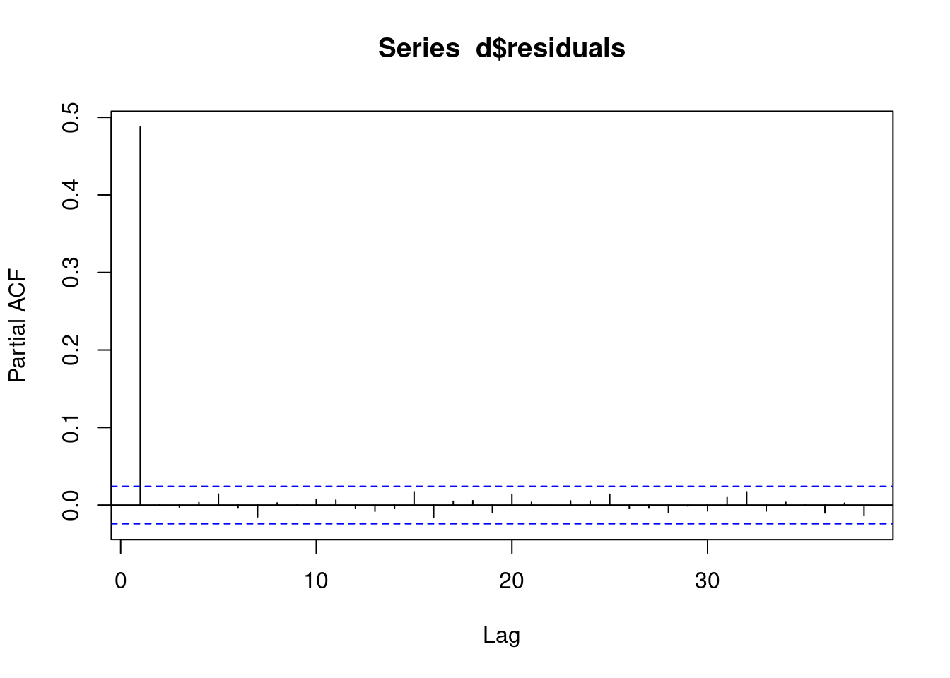
d[,residuals:=residuals(fit1, type ="normalized")]pacf(d$residuals)
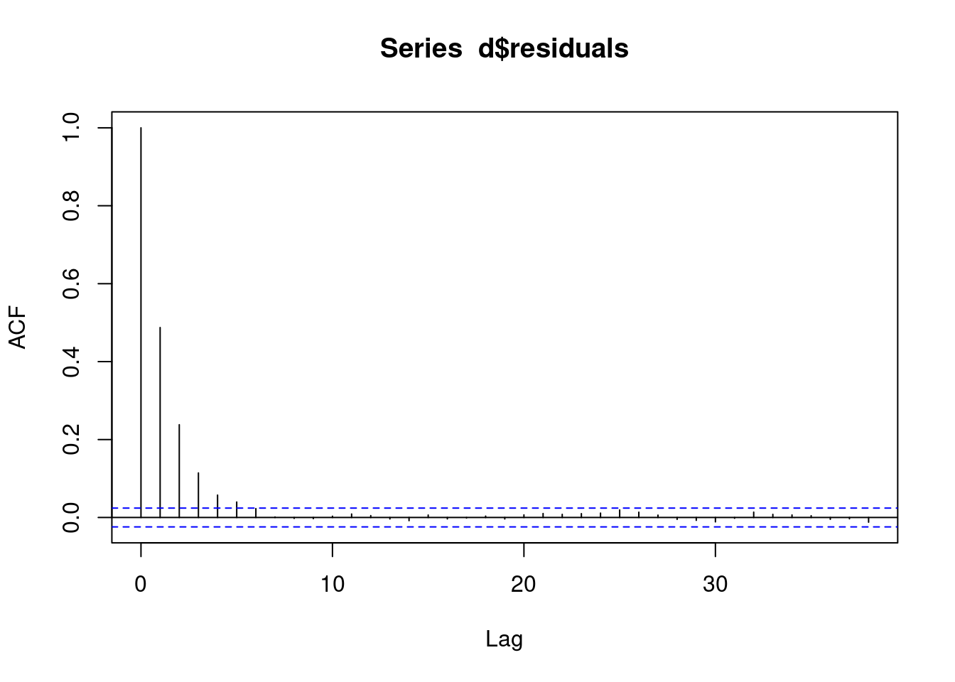
acf(d$residuals)
fit1 <- MASS::glmmPQL(y~season + yearMinus2000 + numberOfCows, random =~1| fylke,family = poisson, data = d,correlation=nlme::corAR1(form=~dayOfSeries|fylke))
iteration 1
iteration 2
iteration 3
summary(fit1)
Linear mixed-effects model fit by maximum likelihood
  Data: d
  AIC BIC logLik
   NA  NA     NA

Random effects:
 Formula: ~1 | fylke
        (Intercept) Residual
StdDev:  0.08328798 1.319938

Correlation Structure: AR(1)
 Formula: ~dayOfSeries | fylke
 Parameter estimate(s):
      Phi
0.5525116
Variance function:
 Structure: fixed weights
 Formula: ~invwt
Fixed effects:  y ~ season + yearMinus2000 + numberOfCows
                   Value  Std.Error   DF   t-value p-value
(Intercept)    0.9283222 0.05561940 6565  16.69062   0.000
seasonSpring   0.8631442 0.01224757 6565  70.47476   0.000
seasonSummer   1.8166993 0.01098229 6565 165.42086   0.000
seasonWinter  -0.1394364 0.01488823 6565  -9.36554   0.000
yearMinus2000  0.2001812 0.00197415 6565 101.40142   0.000
numberOfCows   0.0004206 0.00057695 6565   0.72909   0.466
 Correlation:
              (Intr) ssnSpr ssnSmm ssnWnt yM2000
seasonSpring  -0.155
seasonSummer  -0.171  0.784
seasonWinter  -0.123  0.574  0.621
yearMinus2000 -0.464  0.000  0.000 -0.002
numberOfCows  -0.049  0.001 -0.006  0.004 -0.007

Standardized Within-Group Residuals:
        Min          Q1         Med          Q3         Max
-5.03056012 -0.54478730 -0.04721577  0.46011628 15.05853958

Number of Observations: 6573
Number of Groups: 3
d[,residuals:=residuals(fit1, type ="normalized")]pacf(d$residuals)
acf(d$residuals)
8.3 Exercise 3
library(data.table)d <-fread("data/exercise_3.csv")fit0 <- lme4::glmer(y ~ yearMinus2000 + numberOfCows + (1|fylke), family = poisson, data = d)fit1 <- lme4::glmer(y ~ season + yearMinus2000 + numberOfCows + (1|fylke), family = poisson, data = d)print(lmtest::lrtest(fit0, fit1))
Likelihood ratio test

Model 1: y ~ yearMinus2000 + numberOfCows + (1 | fylke)
Model 2: y ~ season + yearMinus2000 + numberOfCows + (1 | fylke)
  #Df   LogLik Df Chisq Pr(>Chisq)
1   4 -10402.8
2   7  -1830.9  3 17144  < 2.2e-16 ***
---
Signif. codes:  0 '***' 0.001 '**' 0.01 '*' 0.05 '.' 0.1 ' ' 1
summary(fit1)
Generalized linear mixed model fit by maximum likelihood (Laplace
  Approximation) [glmerMod]
 Family: poisson  ( log )
Formula: y ~ season + yearMinus2000 + numberOfCows + (1 | fylke)
   Data: d

     AIC      BIC   logLik deviance df.resid
  3675.9   3706.7  -1830.9   3661.9      593

Scaled residuals:
    Min      1Q  Median      3Q     Max
-3.3420 -0.6168  0.0094  0.5807  3.4186

Random effects:
 Groups Name        Variance Std.Dev.
 fylke  (Intercept) 0.006123 0.07825
Number of obs: 600, groups:  fylke, 3

Fixed effects:
               Estimate Std. Error z value Pr(>|z|)
(Intercept)    0.110463   0.071421   1.547    0.122
seasonSpring   1.005705   0.024761  40.617   <2e-16 ***
seasonSummer   1.995156   0.022578  88.367   <2e-16 ***
seasonWinter  -0.010649   0.030097  -0.354    0.723
yearMinus2000  0.197456   0.003717  53.118   <2e-16 ***
numberOfCows   0.004522   0.002834   1.595    0.111
---
Signif. codes:  0 '***' 0.001 '**' 0.01 '*' 0.05 '.' 0.1 ' ' 1

Correlation of Fixed Effects:
            (Intr) ssnSpr ssnSmm ssnWnt yM2000
seasonSprng -0.276
seasonSummr -0.294  0.792
seasonWintr -0.244  0.595  0.652
yearMns2000 -0.687  0.030  0.030  0.044
numberOfCws -0.193  0.026 -0.002  0.040 -0.015